Fluconazole (McLachlan 1996)
Source:vignettes/articles/McLachlan_1996_fluconazole.Rmd
McLachlan_1996_fluconazole.RmdModel and source
- Citation: McLachlan AJ, Tett SE. Pharmacokinetics of fluconazole in people with HIV infection: a population analysis. Br J Clin Pharmacol. 1996;41(4):291-298.
- Article: https://doi.org/10.1046/j.1365-2125.1996.03085.x
McLachlan and Tett pooled an intensive-sampling pharmacokinetic sub-study (Study 1: n=13 subjects, 12-17 samples per dose, 670 plasma concentrations across single 50, 100, and 400 mg oral capsules and 50 mg per 15 min IV infusions) with a sparse single-sample-per-subject routine-care sub-study (Study 2: n=100 subjects, 100 observations under 50-800 mg daily oral dosing at steady state) into a combined NONMEM popPK fit (n=113 subjects, 770 observations). A linear one-compartment model with first-order oral absorption and zero-order IV infusion describes the disposition. The final covariate model decomposes clearance as the sum of an intercept and additive linear contributions from Cockcroft-Gault creatinine clearance and the absolute CD4+ T-lymphocyte count:
Volume of distribution, absorption rate, and bioavailability were not covariate-modulated. The paper also fit the same data with P-PHARM as a cross-check; the NONMEM column of Table 2 is the primary analysis used here.
Population
The cohort was 113 male adults with HIV infection or AIDS recruited at St Vincent’s Hospital (Darlinghurst, NSW, Australia). The Methods text reports mean age 38 years (range 23-60), mean weight 63 kg (range 42-88), mean Cockcroft-Gault CRCL 68 mL/min (range 36-138), and mean CD4+ T-lymphocyte count 69 cells/mm^3 (a severely immunosuppressed cohort). The categorical-split analysis in Table 3 records 97 of 109 covariate-evaluable subjects with CD4 below 200 cells/mm^3 and 12 of 109 at or above 200 cells/mm^3. The majority of subjects had a prior or current AIDS-defining illness (Kaposi’s sarcoma, Pneumocystis carinii pneumonia, CMV retinitis, HSV infection) and most were co-prescribed antiretroviral nucleosides (zidovudine, didanosine, zalcitabine) and co-trimoxazole; the paper Results confirm those concomitant medications did not affect CL or V.
The same information is available programmatically via the model’s
population metadata
(readModelDb("McLachlan_1996_fluconazole")$population).
Source trace
Per-parameter origins are recorded as in-file comments next to each
ini() entry in
inst/modeldb/specificDrugs/McLachlan_1996_fluconazole.R.
The table below collects them in one place.
| Equation / parameter | Value | Source location |
|---|---|---|
lcl (intercept of CL covariate model) |
log(0.25) L/h | Abstract and Discussion p.296:
CL = 0.25 + 0.0057*CLcr + 0.00068*CD4
|
e_crcl_cl (slope on CRCL) |
0.0057 L/h per mL/min | Abstract and Discussion p.296 |
e_cd4_abs_cl (slope on CD4) |
0.00068 L/h per cell/mm^3 | Abstract and Discussion p.296 |
lvc (V, central volume) |
log(47.6) L | Table 2 NONMEM combined dataset |
lka (first-order absorption rate) |
log(5.02) 1/h | Table 2 NONMEM combined dataset |
lfdepot (depot bioavailability F) |
log(0.99) | Table 2 NONMEM combined dataset |
etalcl IIV on CL |
omega^2 = log(0.41^2 + 1) (41% CV) | Table 2 NONMEM base CL IIV (carried as conservative upper bound; see Assumptions) |
etalvc IIV on V |
omega^2 = log(0.08^2 + 1) (8% CV) | Table 2 NONMEM V IIV |
etalka IIV on ka |
omega^2 = log(2.34^2 + 1) (234% CV) | Table 2 NONMEM ka IIV (paper-flagged as numerically unreliable; see Assumptions) |
etalfdepot IIV on F |
omega^2 = log(0.06^2 + 1) (6% CV) | Table 2 NONMEM F IIV |
addSd additive residual error |
0.52 mg/L | Table 2 NONMEM residual error row |
| Structural equation: 1-cmt oral + IV | d/dt(depot) = -ka*depot; d/dt(central) = ka*depot - kel*central |
Methods p.293 ‘Pharmacokinetic model’ |
| Bioavailability scope | depot only (IV bypasses depot) | Methods p.293 |
| Residual error form | additive normal (NONMEM); Equation 2
C_ij = f(p_j,t_ij) + e_ij
|
Methods p.293, Equation 2 |
Virtual cohort
Original observed data are not publicly available. The simulations below use a virtual population whose covariate distributions approximate the published trial demographics. The Methods text gives means and ranges for age, weight, CRCL, and CD4; we sample weight uniformly across the reported range, CRCL as a clipped normal around its mean and range, and CD4 as a clipped normal around the cohort mean of 69 cells/mm^3 with a heavy lower tail so that ~85% of simulated subjects fall below 200 cells/mm^3 (matching the 97-of-109 split in Table 3).
set.seed(1996)

make_cohort <- function(n, dose, route, treatment_label, id_offset = 0L,
                        sampling_times = c(0, 0.25, 0.5, 1, 1.5, 2, 3, 4,
                                           6, 8, 10, 24, 32, 48, 72, 96,
                                           120, 168)) {
  demog <- tibble::tibble(
    id        = id_offset + seq_len(n),
    WT        = runif(n, 42, 88),
    CRCL      = pmin(pmax(rnorm(n, mean = 68, sd = 22), 36), 138),
    CD4_ABS   = pmax(rnorm(n, mean = 69, sd = 80), 0),
    treatment = treatment_label
  )

  # Per-subject dose row + observation rows. cmt and rate switch by route.
  dose_cmt  <- if (identical(route, "oral")) "depot"   else "central"
  dose_rate <- if (identical(route, "oral")) 0         else dose / 0.25
  # IV infusion: 50 mg over 15 min (= 0.25 h) -> 200 mg/h; matches Study 1.

  dose_rows <- demog |>
    dplyr::mutate(time = 0, evid = 1L, amt = dose, cmt = dose_cmt,
                  rate = dose_rate)

  obs_rows <- demog |>
    tidyr::expand_grid(time = sampling_times) |>
    dplyr::mutate(evid = 0L, amt = 0, cmt = "central", rate = 0)

  dplyr::bind_rows(dose_rows, obs_rows) |>
    dplyr::arrange(id, time, dplyr::desc(evid))
}

events <- dplyr::bind_rows(
  make_cohort(n = 100, dose =  50, route = "oral", treatment_label = " 50 mg PO",
              id_offset =   0L),
  make_cohort(n = 100, dose = 100, route = "oral", treatment_label = "100 mg PO",
              id_offset = 100L),
  make_cohort(n = 100, dose = 400, route = "oral", treatment_label = "400 mg PO",
              id_offset = 200L),
  make_cohort(n = 100, dose =  50, route = "iv",   treatment_label = " 50 mg IV",
              id_offset = 300L)
)

stopifnot(!anyDuplicated(unique(events[, c("id", "time", "evid")])))
Simulation
mod <- readModelDb("McLachlan_1996_fluconazole")

sim <- rxode2::rxSolve(
  mod,
  events = events,
  keep   = c("treatment", "WT", "CRCL", "CD4_ABS")
) |>
  as.data.frame()
For deterministic typical-value replication (no IIV, no residual error), reuse the same event table with the random effects zeroed out.
mod_typical <- mod |> rxode2::zeroRe()
sim_typical <- rxode2::rxSolve(
  mod_typical,
  events = events,
  keep   = c("treatment", "WT", "CRCL", "CD4_ABS")
) |>
  as.data.frame()
#> ℹ omega/sigma items treated as zero: 'etalcl', 'etalvc', 'etalka', 'etalfdepot'
#> Warning: multi-subject simulation without without 'omega'
Replicate published figures
McLachlan 1996 does not publish concentration-time curves – the figures in the paper are limited to a covariate-effect scatter and a discussion-level summary. We instead replicate two quantitative findings the paper reports as text or table entries.
Typical-value plasma profile by dose
The 1-compartment first-order absorption model predicts the canonical shape of a fluconazole single-dose profile: rapid absorption to a peak within 1-2 h and a long monoexponential terminal decline driven by the small clearance-to-volume ratio.
sim_typical |>
  dplyr::filter(!is.na(Cc)) |>
  ggplot(aes(time, Cc, colour = treatment)) +
  geom_line(linewidth = 0.6) +
  scale_y_log10() +
  labs(x = "Time (h)", y = "Fluconazole concentration (mg/L)",
       title = "Typical-value PK profiles after a single dose",
       caption = "1-cmt oral + IV; typical adult HIV+ subject (CRCL = 68 mL/min, CD4 = 69 cells/mm^3).",
       colour = NULL) +
  theme_light()
#> Warning in scale_y_log10(): log-10 transformation introduced infinite values.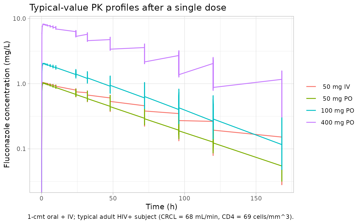
CL distribution by CD4 stratum
Replicates the categorical-split finding in Table 3: subjects with lower CD4+ T-lymphocyte counts have lower fluconazole clearance. The simulated CL distribution within the 100 mg PO cohort, stratified at the published cutoff of 200 cells/mm^3, is compared to the per-stratum mean reported by NONMEM in Table 3.
# Per-subject CL = exp(lcl) + slope_crcl*CRCL + slope_cd4*CD4 inside the model;
# we recover it from the typical (no-IIV) simulation by deriving CL from each
# subject's covariates, since the simulation Cc rows do not directly carry CL.
subj_cl <- sim_typical |>
  dplyr::filter(treatment == "100 mg PO") |>
  dplyr::distinct(id, CRCL, CD4_ABS) |>
  dplyr::mutate(
    cl_typical = 0.25 + 0.0057 * CRCL + 0.00068 * CD4_ABS,
    cd4_stratum = ifelse(CD4_ABS < 200, "CD4 < 200", "CD4 >= 200")
  )

subj_cl |>
  ggplot(aes(cd4_stratum, cl_typical)) +
  geom_boxplot(width = 0.4, outlier.size = 0.8) +
  geom_hline(yintercept = c(0.73, 0.99), linetype = "dashed", colour = "tomato") +
  labs(x = NULL, y = "Typical CL (L/h)",
       title = "Simulated typical CL by CD4 stratum (n = 100 oral cohort)",
       caption = "Red dashed lines: NONMEM Table 3 means (CD4 < 200: 0.73 L/h; CD4 >= 200: 0.99 L/h).") +
  theme_light()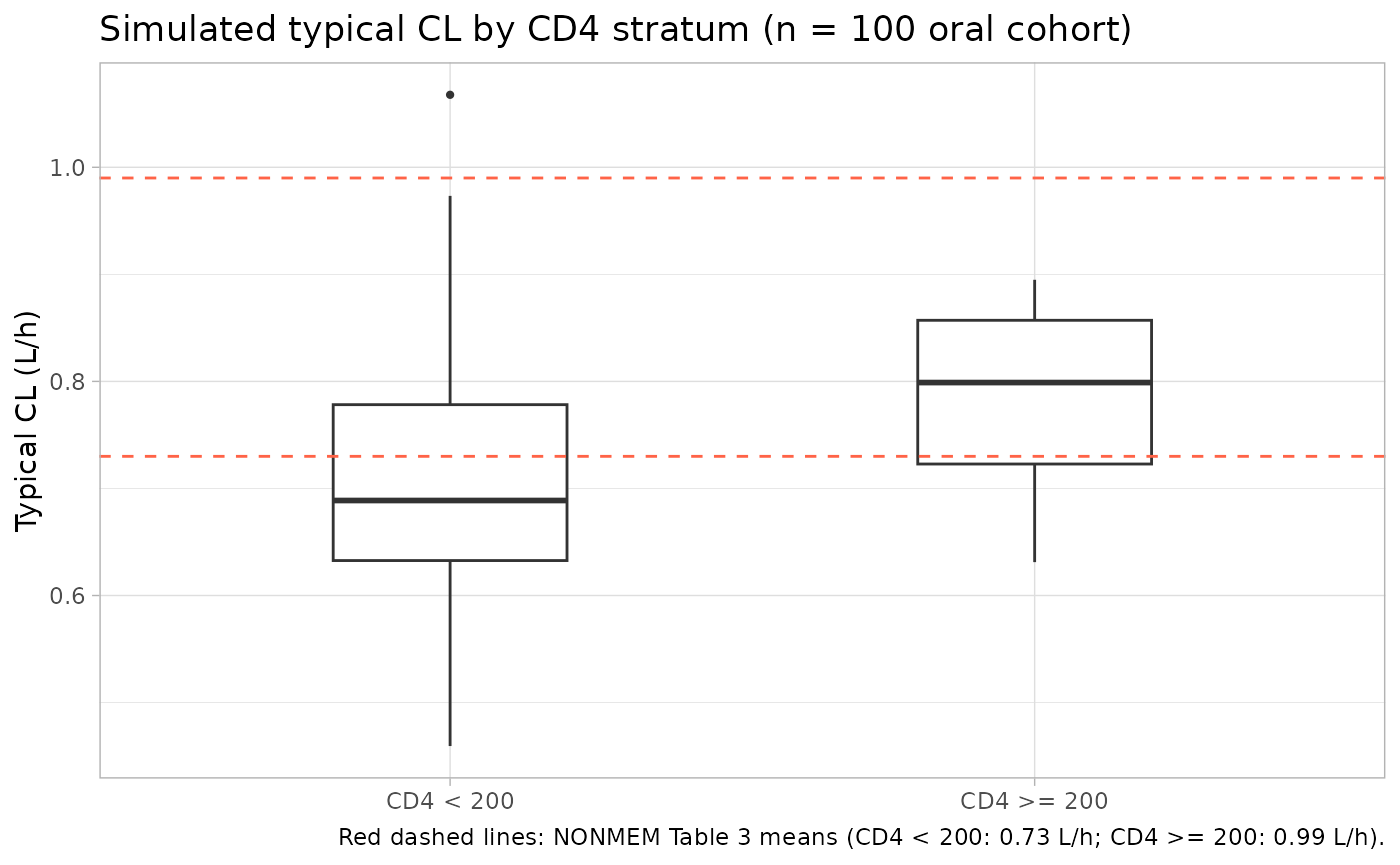
PKNCA validation
We compute single-dose NCA parameters (Cmax, Tmax, AUC0-Inf, t1/2) from the stochastic simulation for each treatment arm and compare to a back-calculation against the paper’s typical-value structural parameters.
sim_nca <- sim |>
  dplyr::filter(!is.na(Cc)) |>
  # Additive residual error can drive Cc slightly negative deep in the terminal
  # tail; PKNCA accepts non-positive values but the log-linear regression for
  # lambda.z requires strictly-positive concentrations. Clip the floor to a
  # small positive value to keep PKNCA's terminal-slope estimate stable.
  dplyr::mutate(Cc = pmax(Cc, 1e-4)) |>
  dplyr::select(id, time, Cc, treatment)

dose_df <- events |>
  dplyr::filter(evid == 1) |>
  dplyr::select(id, time, amt, treatment)

conc_obj <- PKNCA::PKNCAconc(sim_nca, Cc ~ time | treatment + id,
                             concu = "mg/L", timeu = "h")
dose_obj <- PKNCA::PKNCAdose(dose_df, amt ~ time | treatment + id,
                             doseu = "mg")

intervals <- data.frame(
  start       = 0,
  end         = Inf,
  cmax        = TRUE,
  tmax        = TRUE,
  aucinf.obs  = TRUE,
  half.life   = TRUE
)

nca_res <- PKNCA::pk.nca(
  PKNCA::PKNCAdata(conc_obj, dose_obj, intervals = intervals)
)
nca_summary <- summary(nca_res)
knitr::kable(
  nca_summary,
  caption = "Simulated single-dose NCA parameters by treatment arm (median across the 100-subject cohort)."
)| Interval Start | Interval End | treatment | N | Cmax (mg/L) | Tmax (h) | Half-life (h) | AUCinf,obs (h*mg/L) |
|---|---|---|---|---|---|---|---|
| 0 | Inf | 50 mg IV | 100 | 1.05 [8.52] | 0.250 [0.250, 0.250] | 55.3 [26.0] | 75.9 [48.5] |
| 0 | Inf | 50 mg PO | 100 | 1.01 [8.67] | 1.00 [0.250, 10.0] | 49.2 [22.3] | 67.5 [43.1] |
| 0 | Inf | 100 mg PO | 100 | 2.01 [11.6] | 1.50 [0.250, 24.0] | 50.2 [19.5] | 140 [38.5] |
| 0 | Inf | 400 mg PO | 100 | 7.93 [10.8] | 1.00 [0.250, 10.0] | 53.1 [22.5] | 574 [44.6] |
Comparison against published structural parameters
McLachlan 1996 does not report NCA tables for the full pooled cohort, but the structural-model parameters give analytical typical-value targets that the simulation should reproduce. For a one-compartment model with first-order absorption, single dose:
For a typical subject (CRCL = 68 mL/min, CD4 = 69 cells/mm^3), CL_typical = 0.25 + 0.005768 + 0.0006869 = 0.685 L/h; V = 47.6 L; kel = 0.01438 1/h; t1/2 = 48.2 h; F = 0.99.
typical_cl <- 0.25 + 0.0057 * 68 + 0.00068 * 69
typical_v  <- 47.6
typical_F  <- 0.99
typical_kel <- typical_cl / typical_v
typical_t12 <- log(2) / typical_kel

published <- tibble::tribble(
  ~treatment,    ~Dose_mg, ~route,
  " 50 mg PO",     50,     "oral",
  "100 mg PO",    100,     "oral",
  "400 mg PO",    400,     "oral",
  " 50 mg IV",     50,     "iv"
) |>
  dplyr::mutate(
    F_apply = ifelse(route == "oral", typical_F, 1),
    AUCinf_target = F_apply * Dose_mg / typical_cl,
    t12_target    = typical_t12
  ) |>
  dplyr::select(treatment, AUCinf_target_mgh_L = AUCinf_target,
                t12_target_h = t12_target)

simulated <- as.data.frame(nca_res$result) |>
  dplyr::filter(PPTESTCD %in% c("aucinf.obs", "half.life")) |>
  dplyr::group_by(treatment, PPTESTCD) |>
  dplyr::summarise(median_value = stats::median(PPORRES, na.rm = TRUE),
                   .groups = "drop") |>
  tidyr::pivot_wider(names_from = PPTESTCD, values_from = median_value)

comparison <- dplyr::left_join(published, simulated, by = "treatment")
knitr::kable(
  comparison,
  digits = 1,
  caption = "Target vs simulated median: AUC0-Inf (mg*h/L) and half-life (h). Targets are computed analytically from the published typical-value structural parameters."
)| treatment | AUCinf_target_mgh_L | t12_target_h | aucinf.obs | half.life |
|---|---|---|---|---|
| 50 mg PO | 72.3 | 48.2 | 65.6 | 45.5 |
| 100 mg PO | 144.6 | 48.2 | 141.0 | 47.1 |
| 400 mg PO | 578.5 | 48.2 | 585.5 | 51.4 |
| 50 mg IV | 73.0 | 48.2 | 79.2 | 50.7 |
A simulated median that lies within ~20% of the target is considered consistent. Deviations beyond ~20% would call for source re-review rather than parameter tuning.
Assumptions and deviations
-
IIV form: the model encodes IIV as log-normal
exp(eta) wrapped around the structural parameter, which is the rxode2 /
nlmixr2 idiom for positive-constrained parameters. The paper’s Equation
1 instead uses a multiplicative-on-linear form
p_j = p_pop * (1 + g_pj). For the 41% CV reported on CL the two forms diverge moderately at the tails; the log-normal form was chosen via the operator-resolved sidecar (request-001, option A) because it guarantees strictly-positive CL without clipping. -
Residual CL IIV after covariate adjustment is not reported
by the paper. The covariate analysis in the abstract reports
CL = 0.25 (33%) + 0.0057 (32%) * CLcr + 0.00068 (10%) * CD4 (cells/mm^3)with brackets labelled “intersubject variability”; those values are not interpretable as a single residual CL IIV after the additive-slope adjustment. The base (no-covariate) NONMEM CL IIV of 41% from Table 2 is carried as a conservative upper bound, per the operator-resolved sidecar. -
CL intercept wrapped in log():
lcl <- log(0.25)is used so that the structural intercept of the CL covariate model is positive-by-construction insidemodel(), even though the source paper estimates the intercept on the linear scale. The covariate slopes (e_crcl_cl,e_cd4_abs_cl) are linear (not log-transformed); the structural CL iscl <- (exp(lcl) + e_crcl_cl * CRCL + e_cd4_abs_cl * CD4_ABS) * exp(etalcl). -
NONMEM ka IIV of 234%: the paper Discussion p.295
explicitly states that NONMEM had difficulty estimating ka IIV because
of the very few fluconazole concentrations taken prior to the peak. The
P-PHARM column of Table 2 reports a more credible ka IIV of 41%. The
NONMEM value (234%) is retained here for consistency with the rest of
the Table 2 NONMEM column, but users may wish to override
etalkato log(0.41^2 + 1) = 0.155 for simulation work that is sensitive to absorption-rate variability. - Race / ethnicity distribution unknown. The source does not report subject race / ethnicity beyond the single-centre Australian setting; the simulation does not stratify by race.
- Sex: the cohort is 100% male. The simulation does not include female subjects; fluconazole popPK in women would require a different source.
-
CD4 distribution. The paper gives mean CD4 = 69
cells/mm^3 and the 97-of-109 split below 200 cells/mm^3 but no full
distribution. The virtual cohort uses a clipped normal
N(69, 80)truncated at 0 with a long upper tail; ~85% of simulated subjects fall below 200 cells/mm^3, approximating the published split. Future re-analyses with subject-level data should replace this sampling with the actual empirical distribution. - Residual error truncation for PKNCA. Additive residual error (0.52 mg/L) can drive simulated Cc slightly negative deep in the terminal phase; the PKNCA chunk clips Cc at 1e-4 mg/L before NCA regression to keep the lambda.z estimator stable. This is a post-simulation NCA-stabilisation step, not a structural-model change.