Mescaline PK and subjective effects (Mueller 2025)
Source:vignettes/articles/Mueller_2025_mescaline.Rmd
Mueller_2025_mescaline.RmdModel and source
Mescaline is the classic phenethylamine psychedelic of the peyote and San Pedro cacti. Mueller 2025 pooled two randomised, double-blind crossover studies at the University Hospital Basel in which healthy adults took single oral doses of 100 to 800 mg mescaline hydrochloride, and described plasma mescaline, three subjective-effect visual analog scales (VAS) and urinary recovery.
The analysis is a two-stage one: every participant-condition profile was fitted on its own in Phoenix WinNonlin (naive-pooled engine), first the PK and then, with each individual’s PK frozen, the PK-PD. The paper reports summary statistics of the individual estimates (geometric means for PK, Table 2; arithmetic means for PD, Table 3), not a population model. The same PD structure was refitted separately to each of three VAS items, so the paper contributes four model files:
mesc_models <- c(
  "Mueller_2025_mescaline",                # PK only
  "Mueller_2025_mescaline_anydrugeffect",  # PK + 'any drug effect' VAS (primary)
  "Mueller_2025_mescaline_gooddrugeffect", # PK + 'good drug effect' VAS
  "Mueller_2025_mescaline_egodissolution"  # PK + 'ego dissolution' VAS
)
mods <- lapply(stats::setNames(mesc_models, mesc_models), function(m) {
  rxode2::rxode(readModelDb(m))
})- Citation: Mueller L, Klaiber A, Ley L, Becker AM, Thomann J, Luethi D, Schmid Y, Liechti ME (2025). Pharmacokinetics, Pharmacodynamics, and Urinary Recovery of Oral Mescaline Hydrochloride in Healthy Participants. Clin Pharmacokinet 64(10):1495-1506. doi:10.1007/s40262-025-01544-x
- Article: Clin Pharmacokinet 2025;64:1495-1506 (open access)
- Supplement: Electronic Supplementary Material 1 of the article (participant characteristics, exact capsule contents, NCA tables)
for (m in mesc_models) {
  cat(m, "\n", sep = "")
  cat(strwrap(mods[[m]]$description, 76), sep = "\n")
  cat("\n\n")
}
#> Mueller_2025_mescaline
#> One-compartment pharmacokinetic model of oral mescaline (dosed as mescaline
#> hydrochloride capsules) in healthy adults (Mueller 2025), with first-order
#> absorption after an absorption lag time and first-order elimination.
#> Clearance and volume are apparent (Cl/F and Vd/F) because only the oral
#> route was studied; urinary recovery puts the oral bioavailability at 53
#> percent or more. Mueller 2025 fitted every participant-condition profile
#> individually in Phoenix WinNonlin (no population model), so the parameters
#> are the geometric means of 105 individual estimates over all doses (100-800
#> mg mescaline HCl) and the model carries no between-subject variability; the
#> proportional residual error was used but its magnitude was not reported and
#> is fixed at zero. Doses are mg of mescaline base. The effect-compartment
#> sigmoid-Emax PK-PD models for the three subjective-effect scales are
#> Mueller_2025_mescaline_anydrugeffect, _gooddrugeffect and _egodissolution.
#>
#>
#> Mueller_2025_mescaline_anydrugeffect
#> Effect-compartment sigmoid-Emax PK-PD model of the any drug effect visual
#> analog scale (VAS, 0-100 percent) after oral mescaline (dosed as mescaline
#> hydrochloride capsules) in healthy adults (Mueller 2025). Mescaline PK is
#> the one-compartment model with first-order absorption, an absorption lag
#> time and first-order elimination of Mueller_2025_mescaline, held fixed; the
#> effect-site concentration follows plasma with the first-order equilibration
#> rate constant ke0, and the effect is 100 * Ce^gamma / (EC50^gamma +
#> Ce^gamma) with Emax fixed at 100 percent, the top of the scale, and zero
#> baseline. 'Any drug effect' was the primary PD outcome; the same structure
#> was applied to the exploratory 'good drug effect' and 'ego dissolution'
#> scales (Mueller_2025_mescaline_gooddrugeffect, _egodissolution). Mueller
#> 2025 fitted each participant-condition profile individually in Phoenix
#> WinNonlin with the individual PK frozen (no population model); the PD
#> parameters are the arithmetic means of 82 individual estimates over all
#> doses (100-800 mg mescaline HCl; profiles with a predicted maximal effect
#> below 1 percent excluded) and the PK parameters the geometric means of the
#> 105 individual PK estimates. The model therefore carries no between-subject
#> variability; the PK proportional and PD additive residual errors were used
#> but their magnitudes were not reported and are fixed at zero. Doses are mg
#> of mescaline base.
#>
#>
#> Mueller_2025_mescaline_gooddrugeffect
#> Effect-compartment sigmoid-Emax PK-PD model of the good drug effect visual
#> analog scale (VAS, 0-100 percent) after oral mescaline (dosed as mescaline
#> hydrochloride capsules) in healthy adults (Mueller 2025). Mescaline PK is
#> the one-compartment model with first-order absorption, an absorption lag
#> time and first-order elimination of Mueller_2025_mescaline, held fixed; the
#> effect-site concentration follows plasma with the first-order equilibration
#> rate constant ke0, and the effect is 100 * Ce^gamma / (EC50^gamma +
#> Ce^gamma) with Emax fixed at 100 percent, the top of the scale, and zero
#> baseline. The authors regard this scale as exploratory; the primary outcome
#> was 'any drug effect' (Mueller_2025_mescaline_anydrugeffect). Mueller 2025
#> fitted each participant-condition profile individually in Phoenix WinNonlin
#> with the individual PK frozen (no population model); the PD parameters are
#> the arithmetic means of 82 individual estimates over all doses (100-800 mg
#> mescaline HCl; profiles with a predicted maximal effect below 1 percent
#> excluded) and the PK parameters the geometric means of the 105 individual
#> PK estimates. The model therefore carries no between-subject variability;
#> the PK proportional and PD additive residual errors were used but their
#> magnitudes were not reported and are fixed at zero. Doses are mg of
#> mescaline base.
#>
#>
#> Mueller_2025_mescaline_egodissolution
#> Effect-compartment sigmoid-Emax PK-PD model of the ego dissolution visual
#> analog scale (VAS, 0-100 percent) after oral mescaline (dosed as mescaline
#> hydrochloride capsules) in healthy adults (Mueller 2025). Mescaline PK is
#> the one-compartment model with first-order absorption, an absorption lag
#> time and first-order elimination of Mueller_2025_mescaline, held fixed; the
#> effect-site concentration follows plasma with the first-order equilibration
#> rate constant ke0, and the effect is 100 * Ce^gamma / (EC50^gamma +
#> Ce^gamma) with Emax fixed at 100 percent, the top of the scale, and zero
#> baseline. Ego dissolution was rated on the item 'the boundaries between me
#> and my surroundings seem to blur' (5D-ASC item 71); the authors regard it
#> as exploratory, the primary outcome being 'any drug effect'
#> (Mueller_2025_mescaline_anydrugeffect). Mueller 2025 fitted each
#> participant-condition profile individually in Phoenix WinNonlin with the
#> individual PK frozen (no population model); the PD parameters are the
#> arithmetic means of 61 individual estimates over all doses (100-800 mg
#> mescaline HCl; profiles with a predicted maximal effect below 1 percent
#> excluded) and the PK parameters the geometric means of the 105 individual
#> PK estimates. The model therefore carries no between-subject variability;
#> the PK proportional and PD additive residual errors were used but their
#> magnitudes were not reported and are fixed at zero. Doses are mg of
#> mescaline base.
Population
Forty-nine healthy adults (25 women, 24 men; mean age 30 +/- 7 years, weight 70 +/- 9 kg, BMI 22 +/- 2 kg/m^2; supplementary Table S1) took part. Study 1 (NCT04227756) gave 300 mg (n = 16) or 500 mg (n = 16) mescaline HCl in a crossover with LSD, psilocybin and placebo; Study 2 (NCT04849013) gave 17 participants 100, 200, 400 and 800 mg mescaline HCl and 800 mg combined with 40 mg ketanserin. 69 percent had used a psychedelic before. Eight profiles with early emesis were excluded, leaving 105 PK profiles; the ketanserin condition entered the PK analysis only, leaving 91 PK-PD profiles.
str(mods[["Mueller_2025_mescaline"]]$population)
#> List of 13
#>  $ species       : chr "human"
#>  $ n_subjects    : int 49
#>  $ n_studies     : int 2
#>  $ age_range     : chr "25-65 years (inclusion criterion)"
#>  $ age_mean      : chr "30 +/- 7 years"
#>  $ weight_mean   : chr "70 +/- 9 kg"
#>  $ bmi_mean      : chr "22 +/- 2 kg/m^2 (inclusion 18-29 kg/m^2)"
#>  $ sex_female_pct: num 51
#>  $ disease_state : chr "healthy volunteers"
#>  $ dose_range    : chr "Single oral doses of 100, 200, 300, 400, 500 and 800 mg mescaline HCl, and 800 mg mescaline HCl with 40 mg keta"| __truncated__
#>  $ regions       : chr "Switzerland (University Hospital Basel)"
#>  $ n_profiles    : chr "105 PK profiles (113 administrations less 8 with early emesis)"
#>  $ notes         : chr "Supplementary Table S1: 49 participants (25 female) pooled from two randomised double-blind crossover studies ("| __truncated__
Source trace
Each ini() value carries its source location as an
in-file comment. The PK layer is identical in all four files.
| Parameter / equation | Value | Source |
|---|---|---|
lka (ka) |
1.24 1/h | Table 2, ‘All doses’ geometric mean |
ltlag (tlag) |
0.20 h | Table 2, ‘All doses’ |
lcl (Cl/F) |
43 L/h | Table 2, ‘All doses’ |
lvc (Vd/F) |
217 L | Table 2, ‘All doses’ |
propSd |
0 (fixed) | Methods: multiplicative error used, magnitude not reported |
emax |
100 % (fixed) | Methods: ‘an Emax of 100%, according to the range of VASs’ |
lec50, lhill, lke0, any drug
effect |
673 ug/L, 3.5, 1.7 1/h | Table 3, ‘any drug effect’, ‘All doses’ mean |
lec50, lhill, lke0, good drug
effect |
718 ug/L, 3.7, 2.0 1/h | Table 3, ‘good drug effect’, ‘All doses’ mean |
lec50, lhill, lke0, ego
dissolution |
758 ug/L, 8.3, 1.5 1/h | Table 3, ‘ego dissolution’, ‘All doses’ mean |
addSd_<vas> |
0 (fixed) | Methods: additive PD error used, magnitude not reported |
| One compartment, first-order absorption with lag | n/a | Methods ‘PK Analyses and PK-PD Modeling’; Results ‘Model Building’ |
d/dt(effect) <- ke0 * (Cc - effect); sigmoid Emax on
effect
|
n/a | Methods ‘PK Analyses and PK-PD Modeling’ |
| Dose = mescaline-base content of the capsules | n/a | Methods; ESM section 1.3 |
Dosing
Doses were entered as the analytically measured mescaline content (without the HCl) of the capsules (ESM section 1.3), and plasma concentrations are in ug/L.
doses <- tibble::tribble(
  ~condition, ~study, ~dose_hcl, ~dose_base, ~t_end,
  "100 mg",   2,      100,       82.5,       30,
  "200 mg",   2,      200,       164.9,      30,
  "300 mg",   1,      300,       241.6,      24,
  "400 mg",   2,      400,       329.9,      30,
  "500 mg",   1,      500,       404.3,      24,
  "800 mg",   2,      800,       658.3,      30
) |>
  dplyr::mutate(condition = factor(condition, levels = condition))

# Mescaline HCl 247.72 g/mol and base 211.26 g/mol (ESM section 1.4): the
# measured base contents are 85.3 percent of the measured HCl contents.
stopifnot(abs(658.3 / 771.9 - 211.26 / 247.72) < 0.001)

times <- seq(0, 30, by = 1 / 6) # 10-min grid, as the paper's effect NCA

# Observation rows sit on the `central` state with dvid = 1: the PK-PD files
# have two endpoints (Cc and the VAS), and rxode2 returns both outputs at
# every observation row.
make_events <- function(dose_base) {
  dplyr::bind_rows(
    data.frame(id = 1L, time = 0, amt = dose_base, evid = 1L, cmt = "depot", dvid = NA_integer_),
    data.frame(id = 1L, time = times, amt = 0, evid = 0L, cmt = "central", dvid = 1L)
  )
}
The PK layer is the same in every file; check that the four files agree.
Pharmacokinetics
Typical-value secondary parameters
Table 2 derives the secondary parameters from the primary ones in closed form (ke = (Cl/F)/(Vd/F), tmax = ln(ka/ke)/(ka - ke) + tlag, t1/2 = ln 2/ke). Applied to the ‘All doses’ typical values, they reproduce the ‘All doses’ row.
p <- exp(pk_vals[, 1])
ke <- unname(p["lcl"] / p["lvc"])
ka <- unname(p["lka"])
tmax_cf <- log(ka / ke) / (ka - ke) + unname(p["ltlag"])
thalf_cf <- log(2) / ke
c(tmax = tmax_cf, half.life = thalf_cf)
#>      tmax half.life
#>  1.960158  3.497975
# Table 2 'All doses': tmax 2.0 h, t1/2 3.5 h (each printed to 2 significant digits).
stopifnot(abs(tmax_cf - 2.0) < 0.05, abs(thalf_cf - 3.5) < 0.05)
Per-dose replication of Table 2
Table 2 also lists the geometric-mean primary parameters for each dose. Solving the model with each dose’s own primary parameters and running PKNCA on the solved profile should return that dose’s secondary parameters. This checks the model structure, the dose input (mescaline base) and the concentration units together. The paper’s secondary values are geometric means of individual secondary values, which differ slightly from the value at the geometric-mean parameters, so small differences are expected.
tab2 <- tibble::tribble(
  ~condition, ~ka,  ~tlag, ~cl, ~vc, ~cmax, ~tmax, ~aucinf.obs, ~half.life,
  "100 mg",   2.59, 0.19,  46,  225, 284,   1.3,   1803,        3.4,
  "200 mg",   1.67, 0.25,  46,  233, 521,   1.7,   3553,        3.5,
  "300 mg",   0.96, 0.15,  37,  191, 826,   2.2,   6533,        3.6,
  "400 mg",   1.10, 0.17,  43,  223, 1001,  2.1,   7575,        3.6,
  "500 mg",   0.80, 0.18,  45,  214, 1124,  2.4,   9037,        3.3,
  "800 mg",   0.74, 0.19,  42,  220, 1778,  2.6,   15765,       3.7
)

solve_pk <- function(cond, params = NULL) {
  d <- doses[doses$condition == cond, ]
  ev <- make_events(d$dose_base)
  s <- if (is.null(params)) {
    rxode2::rxSolve(mods[["Mueller_2025_mescaline"]], ev)
  } else {
    rxode2::rxSolve(mods[["Mueller_2025_mescaline"]], ev, params = params)
  }
  as.data.frame(s) |>
    dplyr::mutate(condition = cond, id = match(cond, levels(doses$condition)))
}

sim_perdose <- dplyr::bind_rows(lapply(tab2$condition, function(cond) {
  r <- tab2[tab2$condition == cond, ]
  solve_pk(cond, params = c(
    lka = log(r$ka), ltlag = log(r$tlag), lcl = log(r$cl), lvc = log(r$vc)
  ))
}))
sim_typical <- dplyr::bind_rows(lapply(as.character(doses$condition), solve_pk))
run_nca <- function(sim) {
  conc <- sim |>
    dplyr::filter(!is.na(Cc)) |>
    dplyr::mutate(Cc = pmax(Cc, 0)) |>
    dplyr::select(id, time, Cc, condition)
  conc <- dplyr::bind_rows(
    conc,
    conc |> dplyr::distinct(id, condition) |> dplyr::mutate(time = 0, Cc = 0)
  ) |>
    dplyr::distinct(id, condition, time, .keep_all = TRUE) |>
    dplyr::arrange(id, condition, time)
  dose_df <- doses |>
    dplyr::mutate(
      id = match(as.character(condition), levels(condition)),
      condition = as.character(condition), time = 0, amt = dose_base
    ) |>
    dplyr::select(id, time, amt, condition)
  conc_obj <- PKNCA::PKNCAconc(conc, Cc ~ time | condition + id)
  dose_obj <- PKNCA::PKNCAdose(dose_df, amt ~ time | condition + id)
  intervals <- data.frame(
    start = 0, end = Inf,
    cmax = TRUE, tmax = TRUE, aucinf.obs = TRUE, half.life = TRUE
  )
  PKNCA::pk.nca(PKNCA::PKNCAdata(conc_obj, dose_obj, intervals = intervals))
}

nca_perdose <- run_nca(sim_perdose)
cmp_perdose <- nlmixr2lib::ncaComparisonTable(
  simulated = nca_perdose,
  reference = tab2 |> dplyr::select(condition, cmax, tmax, aucinf.obs, half.life),
  by = "condition",
  units = c(cmax = "ug/L", tmax = "h", aucinf.obs = "h*ug/L", half.life = "h"),
  tolerance_pct = 20
)
knitr::kable(
  cmp_perdose,
  caption = paste(
    "Model solved with each dose's Table 2 primary parameters vs the Table 2",
    "secondary parameters. * differs from the reference by more than 20%."
  )
)| NCA parameter | condition | Reference | Simulated | % diff |
|---|---|---|---|---|
| Cmax (ug/L) | 100 mg | 284 | 295 | +3.7% |
| Cmax (ug/L) | 200 mg | 521 | 531 | +2.0% |
| Cmax (ug/L) | 300 mg | 826 | 844 | +2.1% |
| Cmax (ug/L) | 400 mg | 1000 | 1020 | +2.0% |
| Cmax (ug/L) | 500 mg | 1120 | 1170 | +4.4% |
| Cmax (ug/L) | 800 mg | 1780 | 1870 | +5.1% |
| Tmax (h) | 100 mg | 1.3 | 1.33 | +2.6% |
| Tmax (h) | 200 mg | 1.7 | 1.67 | -2.0% |
| Tmax (h) | 300 mg | 2.2 | 2.17 | -1.5% |
| Tmax (h) | 400 mg | 2.1 | 2.17 | +3.2% |
| Tmax (h) | 500 mg | 2.4 | 2.5 | +4.2% |
| Tmax (h) | 800 mg | 2.6 | 2.67 | +2.6% |
| AUC0-∞ (obs) (h*ug/L) | 100 mg | 1800 | 1790 | -0.6% |
| AUC0-∞ (obs) (h*ug/L) | 200 mg | 3550 | 3590 | +0.9% |
| AUC0-∞ (obs) (h*ug/L) | 300 mg | 6530 | 6530 | -0.1% |
| AUC0-∞ (obs) (h*ug/L) | 400 mg | 7580 | 7670 | +1.2% |
| AUC0-∞ (obs) (h*ug/L) | 500 mg | 9040 | 8980 | -0.6% |
| AUC0-∞ (obs) (h*ug/L) | 800 mg | 15800 | 15700 | -0.6% |
| t½ (h) | 100 mg | 3.4 | 3.39 | -0.2% |
| t½ (h) | 200 mg | 3.5 | 3.52 | +0.6% |
| t½ (h) | 300 mg | 3.6 | 3.6 | -0.1% |
| t½ (h) | 400 mg | 3.6 | 3.61 | +0.3% |
| t½ (h) | 500 mg | 3.3 | 3.32 | +0.5% |
| t½ (h) | 800 mg | 3.7 | 3.66 | -1.2% |
nca_pd_df <- as.data.frame(nca_perdose) |>
  dplyr::filter(PPTESTCD %in% c("cmax", "aucinf.obs", "half.life")) |>
  dplyr::select(condition, PPTESTCD, PPORRES) |>
  dplyr::left_join(
    tab2 |>
      dplyr::select(condition, cmax, aucinf.obs, half.life) |>
      tidyr::pivot_longer(-condition, names_to = "PPTESTCD", values_to = "ref"),
    by = c("condition", "PPTESTCD")
  ) |>
  dplyr::mutate(pct_diff = 100 * (PPORRES / ref - 1))
# AUC = Dose/(Cl/F) and t1/2 = ln 2/ke are exact functions of the primary
# parameters (the paper's AUC needs Dose = mescaline base, so a wrong salt
# factor shows here as a 17% error); Cmax depends on ka, whose geometric mean
# does not commute with the Cmax formula, hence the wider Cmax bound.
stopifnot(
  all(abs(nca_pd_df$pct_diff[nca_pd_df$PPTESTCD == "aucinf.obs"]) < 3),
  all(abs(nca_pd_df$pct_diff[nca_pd_df$PPTESTCD == "half.life"]) < 6),
  all(abs(nca_pd_df$pct_diff[nca_pd_df$PPTESTCD == "cmax"]) < 10)
)
Concentration-time profiles (Figure 1a)
dplyr::bind_rows(
  sim_typical |> dplyr::mutate(set = "All-doses typical value"),
  sim_perdose |> dplyr::mutate(set = "Per-dose Table 2 parameters")
) |>
  dplyr::mutate(condition = factor(condition, levels = levels(doses$condition))) |>
  ggplot(aes(time, Cc, colour = condition, linetype = set)) +
  geom_line() +
  labs(x = "Time (h)", y = "Mescaline (ug/L)", colour = "Dose (HCl)", linetype = NULL) +
  theme_bw()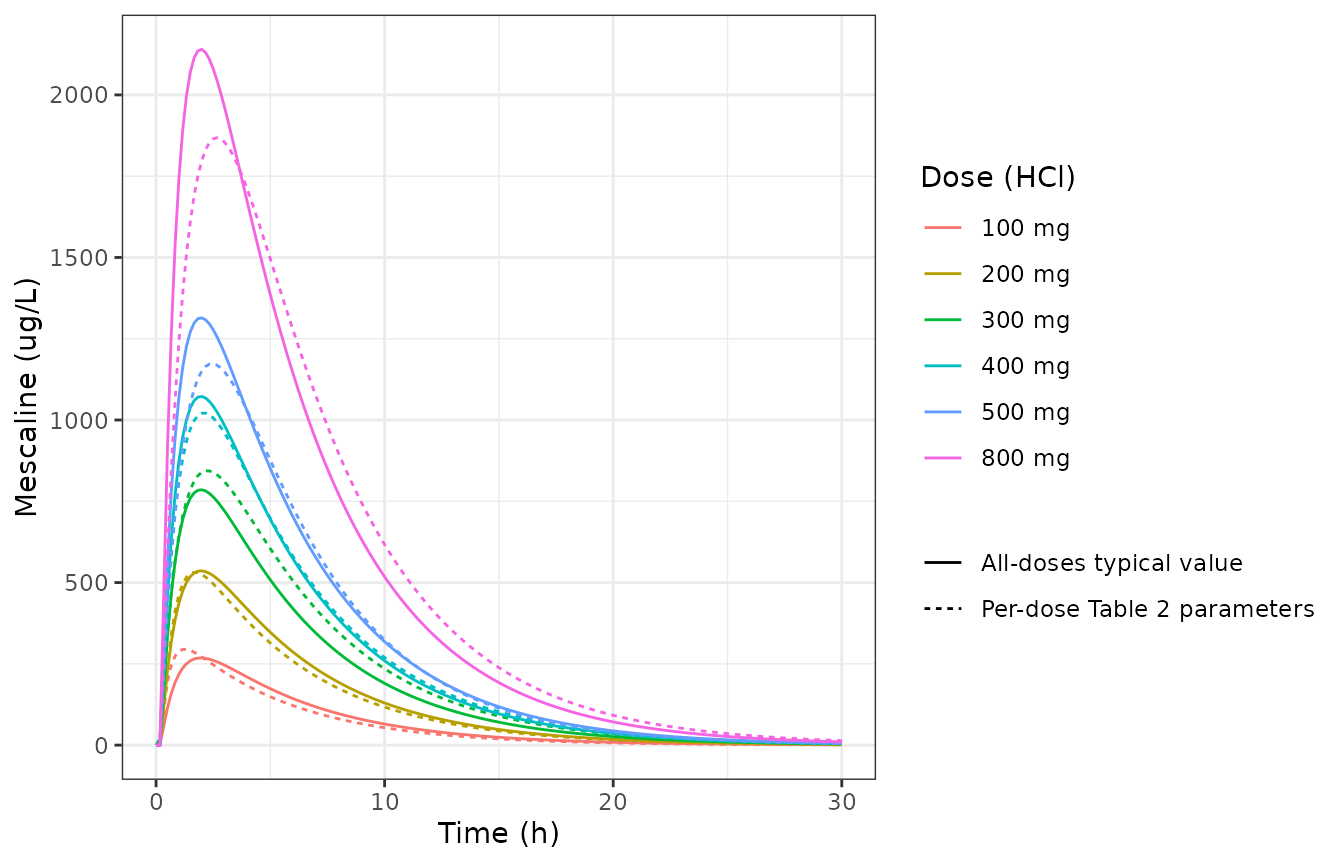
Replicates Figure 1a of Mueller 2025: mescaline plasma concentration by dose. Solid: typical-value model (All-doses parameters); dashed: each dose’s own Table 2 geometric-mean parameters. The published panel shows the geometric mean of the individual predicted curves.
PKNCA of the typical-value model
The typical-value model (one set of parameters for all doses) against the per-dose Table 2 secondary parameters. Mueller 2025 found exposure dose proportional, but the per-dose geometric-mean ka falls from 2.6 1/h at 100 mg to 0.7 1/h at 800 mg; one typical ka over-predicts Cmax and under-predicts tmax at the high doses and does the reverse at 100 mg. AUC and half-life are dose-independent in the model and follow Table 2 to within the dose-to-dose scatter of Cl/F (37 to 46 L/h).
nca_typical <- run_nca(sim_typical)
cmp_typical <- nlmixr2lib::ncaComparisonTable(
  simulated = nca_typical,
  reference = tab2 |> dplyr::select(condition, cmax, tmax, aucinf.obs, half.life),
  by = "condition",
  units = c(cmax = "ug/L", tmax = "h", aucinf.obs = "h*ug/L", half.life = "h"),
  tolerance_pct = 20
)
knitr::kable(
  cmp_typical,
  caption = paste(
    "Typical-value model (All-doses parameters) vs Table 2 per-dose secondary",
    "parameters. * differs from the reference by more than 20%."
  )
)| NCA parameter | condition | Reference | Simulated | % diff |
|---|---|---|---|---|
| Cmax (ug/L) | 100 mg | 284 | 268 | -5.6% |
| Cmax (ug/L) | 200 mg | 521 | 536 | +2.9% |
| Cmax (ug/L) | 300 mg | 826 | 785 | -4.9% |
| Cmax (ug/L) | 400 mg | 1000 | 1070 | +7.1% |
| Cmax (ug/L) | 500 mg | 1120 | 1310 | +16.9% |
| Cmax (ug/L) | 800 mg | 1780 | 2140 | +20.4%* |
| Tmax (h) | 100 mg | 1.3 | 2 | +53.8%* |
| Tmax (h) | 200 mg | 1.7 | 2 | +17.6% |
| Tmax (h) | 300 mg | 2.2 | 2 | -9.1% |
| Tmax (h) | 400 mg | 2.1 | 2 | -4.8% |
| Tmax (h) | 500 mg | 2.4 | 2 | -16.7% |
| Tmax (h) | 800 mg | 2.6 | 2 | -23.1%* |
| AUC0-∞ (obs) (h*ug/L) | 100 mg | 1800 | 1920 | +6.4% |
| AUC0-∞ (obs) (h*ug/L) | 200 mg | 3550 | 3830 | +7.9% |
| AUC0-∞ (obs) (h*ug/L) | 300 mg | 6530 | 5620 | -14.0% |
| AUC0-∞ (obs) (h*ug/L) | 400 mg | 7580 | 7670 | +1.3% |
| AUC0-∞ (obs) (h*ug/L) | 500 mg | 9040 | 9400 | +4.0% |
| AUC0-∞ (obs) (h*ug/L) | 800 mg | 15800 | 15300 | -2.9% |
| t½ (h) | 100 mg | 3.4 | 3.51 | +3.3% |
| t½ (h) | 200 mg | 3.5 | 3.51 | +0.4% |
| t½ (h) | 300 mg | 3.6 | 3.51 | -2.4% |
| t½ (h) | 400 mg | 3.6 | 3.51 | -2.4% |
| t½ (h) | 500 mg | 3.3 | 3.51 | +6.5% |
| t½ (h) | 800 mg | 3.7 | 3.51 | -5.1% |
Subjective effects
Effect metrics
Mueller 2025 summarised each VAS with an NCA of the model-predicted effect-time curve on a 10-min grid: Emax and its time tmaxE, the area under the effect curve (AUEC, linear trapezoid, to the end of sampling at 24 or 30 h), and onset and duration defined by a threshold of 10% of the profile’s Emax. The helper below computes the same quantities, with PKNCA for the AUEC.
vas <- c(
  Mueller_2025_mescaline_anydrugeffect = "anydrugeffectvas",
  Mueller_2025_mescaline_gooddrugeffect = "gooddrugeffectvas",
  Mueller_2025_mescaline_egodissolution = "egodissolutionvas"
)
vas_label <- c(
  anydrugeffectvas = "Any drug effect",
  gooddrugeffectvas = "Good drug effect",
  egodissolutionvas = "Ego dissolution"
)

solve_pd <- function(model_name, cond, params = NULL) {
  d <- doses[doses$condition == cond, ]
  ev <- make_events(d$dose_base)
  s <- if (is.null(params)) {
    rxode2::rxSolve(mods[[model_name]], ev)
  } else {
    rxode2::rxSolve(mods[[model_name]], ev, params = params)
  }
  out <- as.data.frame(s)
  data.frame(
    time = out$time, Cc = out$Cc, effect = out[[vas[[model_name]]]],
    scale = vas[[model_name]], condition = cond,
    id = match(cond, levels(doses$condition)), t_end = d$t_end
  )
}

effect_metrics <- function(sim) {
  sim <- sim |> dplyr::filter(time <= t_end)
  # AUEC by PKNCA, linear trapezoid over 0 to the end of sampling.
  auec <- dplyr::bind_rows(lapply(split(sim, list(sim$scale, sim$condition), drop = TRUE), function(d) {
    co <- PKNCA::PKNCAconc(d, effect ~ time | scale + condition + id)
    iv <- data.frame(start = 0, end = d$t_end[1], auclast = TRUE)
    r <- PKNCA::pk.nca(PKNCA::PKNCAdata(co, intervals = iv,
                                       options = list(auc.method = "linear")))
    as.data.frame(r) |>
      dplyr::filter(PPTESTCD == "auclast") |>
      dplyr::transmute(scale, condition, AUEC = PPORRES)
  }))
  thr <- sim |>
    dplyr::group_by(scale, condition) |>
    dplyr::summarise(
      Emax = max(effect),
      tmaxE = time[which.max(effect)],
      tonset = min(time[effect >= 0.1 * max(effect)]),
      toffset = max(time[effect >= 0.1 * max(effect)]),
      .groups = "drop"
    ) |>
    dplyr::mutate(duration = toffset - tonset) |>
    dplyr::select(-toffset)
  dplyr::left_join(thr, auec, by = c("scale", "condition"))
}
tab3 <- tibble::tribble(
  ~scale,              ~condition, ~ec50, ~hill, ~ke0, ~AUEC, ~Emax, ~tonset, ~tmaxE, ~duration,
  "anydrugeffectvas",  "100 mg",   506,   3.8,   2.5,  44,    13,    0.8,     1.9,    2.8,
  "anydrugeffectvas",  "200 mg",   687,   2.8,   1.6,  157,   30,    0.9,     2.9,    7.1,
  "anydrugeffectvas",  "300 mg",   712,   3.8,   1.7,  321,   52,    1.3,     3.5,    8.0,
  "anydrugeffectvas",  "400 mg",   844,   2.9,   1.8,  383,   58,    0.8,     3.1,    9.8,
  "anydrugeffectvas",  "500 mg",   602,   4.9,   1.3,  608,   80,    1.4,     4.2,    10,
  "anydrugeffectvas",  "800 mg",   680,   3.0,   1.6,  948,   89,    0.7,     3.8,    15,
  "gooddrugeffectvas", "100 mg",   495,   4.3,   3.3,  68,    18,    0.9,     1.8,    2.6,
  "gooddrugeffectvas", "200 mg",   737,   3.3,   1.2,  194,   35,    0.9,     2.8,    7.4,
  "gooddrugeffectvas", "300 mg",   794,   4.8,   1.8,  333,   48,    1.5,     4.1,    8.0,
  "gooddrugeffectvas", "400 mg",   933,   2.8,   2.1,  395,   56,    0.8,     3.0,    9.9,
  "gooddrugeffectvas", "500 mg",   570,   4.7,   1.4,  665,   72,    1.2,     3.6,    11,
  "gooddrugeffectvas", "800 mg",   733,   2.6,   2.4,  925,   81,    0.8,     4.1,    15,
  "egodissolutionvas", "100 mg",   359,   9.0,   2.1,  7.6,   2.8,   1.7,     0.7,    0.5,
  "egodissolutionvas", "200 mg",   525,   7.0,   1.4,  49,    13,    2.2,     2.2,    2.5,
  "egodissolutionvas", "300 mg",   742,   11,    2.1,  153,   38,    1.8,     2.6,    3.4,
  "egodissolutionvas", "400 mg",   921,   7.1,   1.4,  171,   38,    1.7,     3.3,    4.4,
  "egodissolutionvas", "500 mg",   876,   11,    1.1,  230,   53,    2.2,     3.4,    4.1,
  "egodissolutionvas", "800 mg",   834,   4.3,   1.4,  800,   90,    1.0,     4.1,    12
)

sim_pd_typical <- dplyr::bind_rows(lapply(names(vas), function(m) {
  dplyr::bind_rows(lapply(as.character(doses$condition), function(cond) solve_pd(m, cond)))
}))

sim_pd_perdose <- dplyr::bind_rows(lapply(names(vas), function(m) {
  dplyr::bind_rows(lapply(as.character(doses$condition), function(cond) {
    r2 <- tab2[tab2$condition == cond, ]
    r3 <- tab3[tab3$scale == vas[[m]] & tab3$condition == cond, ]
    solve_pd(m, cond, params = c(
      lka = log(r2$ka), ltlag = log(r2$tlag), lcl = log(r2$cl), lvc = log(r2$vc),
      lec50 = log(r3$ec50), lhill = log(r3$hill), lke0 = log(r3$ke0)
    ))
  }))
}))

met_typical <- effect_metrics(sim_pd_typical)
#> No dose information provided, calculations requiring dose will return NA.
#> No dose information provided, calculations requiring dose will return NA.
#> No dose information provided, calculations requiring dose will return NA.
#> No dose information provided, calculations requiring dose will return NA.
#> No dose information provided, calculations requiring dose will return NA.
#> No dose information provided, calculations requiring dose will return NA.
#> No dose information provided, calculations requiring dose will return NA.
#> No dose information provided, calculations requiring dose will return NA.
#> No dose information provided, calculations requiring dose will return NA.
#> No dose information provided, calculations requiring dose will return NA.
#> No dose information provided, calculations requiring dose will return NA.
#> No dose information provided, calculations requiring dose will return NA.
#> No dose information provided, calculations requiring dose will return NA.
#> No dose information provided, calculations requiring dose will return NA.
#> No dose information provided, calculations requiring dose will return NA.
#> No dose information provided, calculations requiring dose will return NA.
#> No dose information provided, calculations requiring dose will return NA.
#> No dose information provided, calculations requiring dose will return NA.
met_perdose <- effect_metrics(sim_pd_perdose)
#> No dose information provided, calculations requiring dose will return NA.
#> No dose information provided, calculations requiring dose will return NA.
#> No dose information provided, calculations requiring dose will return NA.
#> No dose information provided, calculations requiring dose will return NA.
#> No dose information provided, calculations requiring dose will return NA.
#> No dose information provided, calculations requiring dose will return NA.
#> No dose information provided, calculations requiring dose will return NA.
#> No dose information provided, calculations requiring dose will return NA.
#> No dose information provided, calculations requiring dose will return NA.
#> No dose information provided, calculations requiring dose will return NA.
#> No dose information provided, calculations requiring dose will return NA.
#> No dose information provided, calculations requiring dose will return NA.
#> No dose information provided, calculations requiring dose will return NA.
#> No dose information provided, calculations requiring dose will return NA.
#> No dose information provided, calculations requiring dose will return NA.
#> No dose information provided, calculations requiring dose will return NA.
#> No dose information provided, calculations requiring dose will return NA.
#> No dose information provided, calculations requiring dose will return NA.
Effect-time curves (Figure 1b-d and Figure 2)
dplyr::bind_rows(
  sim_pd_typical |> dplyr::mutate(set = "All-doses typical value"),
  sim_pd_perdose |> dplyr::mutate(set = "Per-dose Table 2/3 parameters")
) |>
  dplyr::mutate(
    condition = factor(condition, levels = levels(doses$condition)),
    scale = factor(vas_label[scale], levels = vas_label)
  ) |>
  ggplot(aes(time, effect, colour = condition, linetype = set)) +
  geom_line() +
  facet_wrap(~scale, ncol = 1) +
  coord_cartesian(ylim = c(0, 100)) +
  labs(x = "Time (h)", y = "Predicted effect (%)", colour = "Dose (HCl)", linetype = NULL) +
  theme_bw()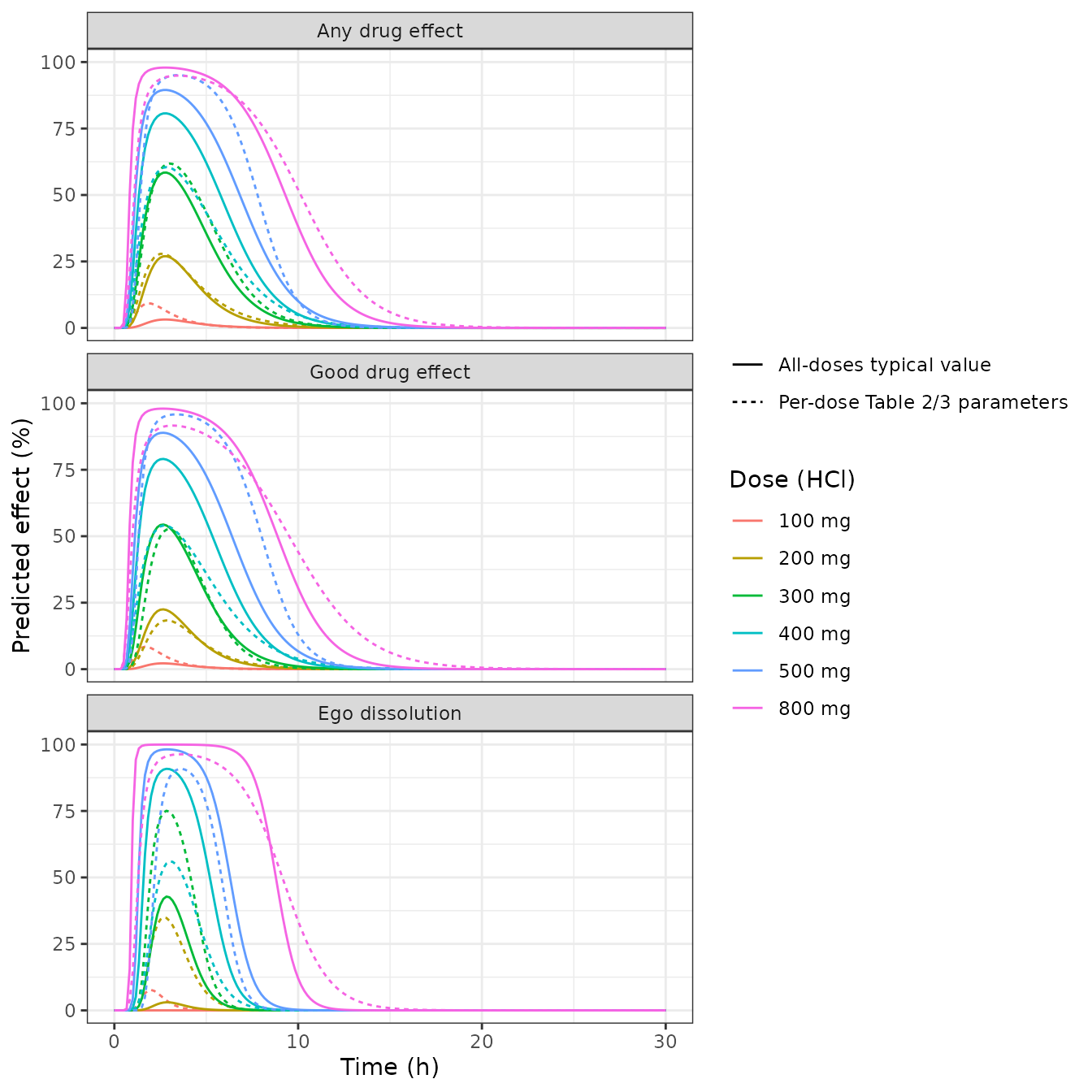
Replicates Figure 1b-d of Mueller 2025: predicted VAS effect by dose. Solid: typical-value model (All-doses parameters); dashed: each dose’s own Table 2 and Table 3 mean parameters. The published panels show the arithmetic mean of the individual predicted curves.
Comparison with Table 3
cmp3 <- met_typical |>
  dplyr::rename_with(~ paste0(.x, "_typ"), c(Emax, tmaxE, tonset, duration, AUEC)) |>
  dplyr::left_join(
    met_perdose |>
      dplyr::rename_with(~ paste0(.x, "_pd"), c(Emax, tmaxE, tonset, duration, AUEC)),
    by = c("scale", "condition")
  ) |>
  dplyr::left_join(
    tab3 |> dplyr::select(scale, condition, Emax, tmaxE, tonset, duration, AUEC),
    by = c("scale", "condition")
  ) |>
  dplyr::mutate(scale = factor(vas_label[scale], levels = vas_label)) |>
  dplyr::arrange(scale, condition)

cmp3 |>
  dplyr::transmute(
    scale, condition,
    Emax_typ = round(Emax_typ), Emax_pd = round(Emax_pd), Emax,
    tmaxE_typ = round(tmaxE_typ, 1), tmaxE_pd = round(tmaxE_pd, 1), tmaxE,
    AUEC_typ = round(AUEC_typ), AUEC_pd = round(AUEC_pd), AUEC
  ) |>
  dplyr::rename(
    "VAS" = scale, "Dose (HCl)" = condition,
    "Emax typical (%)" = Emax_typ, "Emax per-dose (%)" = Emax_pd, "Emax Table 3 (%)" = Emax,
    "tmaxE typical (h)" = tmaxE_typ, "tmaxE per-dose (h)" = tmaxE_pd, "tmaxE Table 3 (h)" = tmaxE,
    "AUEC typical (h*%)" = AUEC_typ, "AUEC per-dose (h*%)" = AUEC_pd, "AUEC Table 3 (h*%)" = AUEC
  ) |>
  knitr::kable(caption = paste(
    "Effect metrics of the typical-value curve (All-doses parameters), of the",
    "curve at each dose's own mean parameters, and the Table 3 means of the",
    "individual predicted curves."
))| VAS | Dose (HCl) | Emax typical (%) | Emax per-dose (%) | Emax Table 3 (%) | tmaxE typical (h) | tmaxE per-dose (h) | tmaxE Table 3 (h) | AUEC typical (h*%) | AUEC per-dose (h*%) | AUEC Table 3 (h*%) |
|---|---|---|---|---|---|---|---|---|---|---|
| Any drug effect | 100 mg | 3 | 9 | 13.0 | 2.8 | 1.8 | 1.9 | 11 | 23 | 44.0 |
| Any drug effect | 200 mg | 27 | 28 | 30.0 | 2.8 | 2.7 | 2.9 | 98 | 112 | 157.0 |
| Any drug effect | 300 mg | 58 | 62 | 52.0 | 2.8 | 3.0 | 3.5 | 253 | 283 | 321.0 |
| Any drug effect | 400 mg | 81 | 60 | 58.0 | 2.8 | 2.8 | 3.1 | 430 | 311 | 383.0 |
| Any drug effect | 500 mg | 89 | 95 | 80.0 | 2.8 | 3.5 | 4.2 | 553 | 615 | 608.0 |
| Any drug effect | 800 mg | 98 | 95 | 89.0 | 2.8 | 3.5 | 3.8 | 838 | 884 | 948.0 |
| Good drug effect | 100 mg | 2 | 8 | 18.0 | 2.7 | 1.7 | 1.8 | 7 | 19 | 68.0 |
| Good drug effect | 200 mg | 22 | 18 | 35.0 | 2.7 | 2.8 | 2.8 | 76 | 68 | 194.0 |
| Good drug effect | 300 mg | 54 | 53 | 48.0 | 2.7 | 3.0 | 4.1 | 216 | 196 | 333.0 |
| Good drug effect | 400 mg | 79 | 54 | 56.0 | 2.7 | 2.7 | 3.0 | 390 | 268 | 395.0 |
| Good drug effect | 500 mg | 89 | 96 | 72.0 | 2.7 | 3.3 | 3.6 | 513 | 649 | 665.0 |
| Good drug effect | 800 mg | 98 | 92 | 81.0 | 2.7 | 3.2 | 4.1 | 798 | 830 | 925.0 |
| Ego dissolution | 100 mg | 0 | 8 | 2.8 | 2.8 | 2.0 | 0.7 | 0 | 12 | 7.6 |
| Ego dissolution | 200 mg | 3 | 35 | 13.0 | 2.8 | 2.7 | 2.2 | 6 | 86 | 49.0 |
| Ego dissolution | 300 mg | 43 | 75 | 38.0 | 2.8 | 2.8 | 2.6 | 104 | 203 | 153.0 |
| Ego dissolution | 400 mg | 91 | 56 | 38.0 | 2.8 | 3.0 | 3.3 | 342 | 170 | 171.0 |
| Ego dissolution | 500 mg | 98 | 91 | 53.0 | 2.8 | 3.7 | 3.4 | 489 | 341 | 230.0 |
| Ego dissolution | 800 mg | 100 | 96 | 90.0 | 2.8 | 3.7 | 4.1 | 783 | 764 | 800.0 |
Table 3 reports the mean of individual metrics, while the model gives the metric of a single typical curve. With a steep sigmoid (gamma 3.5 to 8.3) these differ systematically. At low doses the typical effect-site concentration sits well below EC50 and the typical curve is small, but the more sensitive or higher-exposure individuals contribute large effects to the mean, so the typical curve falls below the published mean at 100-200 mg. At the high doses the typical curve is close to the 100% ceiling, while the less sensitive individuals pull the published mean down, so the typical curve lies above it (98% against 89% for ‘any drug effect’ at 800 mg). The typical curve is therefore steeper in dose than the published mean, and most so for ‘ego dissolution’ (gamma 8.3). Its peak time is the same at every dose (2.8 h), because the PK is linear and one ka serves all doses; the published tmaxE rises with dose, following the slower absorption estimated at the higher doses. Each dose’s own Table 2 and Table 3 parameters bring the curve closer to the published mean at most doses but not at all of them, because the published mean is still a mean over individuals. This is how a typical-value model behaves in a steep nonlinear PD system, not a transcription error. The checks below test what a typical curve should reproduce.
any_typ <- met_typical |> dplyr::filter(scale == "anydrugeffectvas")
# 1. Dose ordering: the typical effect peak rises with dose for every scale.
for (s in names(vas_label)) {
  e <- met_typical$Emax[met_typical$scale == s]
  stopifnot(all(diff(e[order(match(met_typical$condition[met_typical$scale == s],
                                   levels(doses$condition)))]) > 0))
}
# 2. Overall effect exposure: at 300-800 mg, where the typical effect-site
#    concentration reaches EC50, the typical 'any drug effect' AUEC must track
#    the Table 3 mean. A typical curve differs from a mean of individual
#    curves by some tens of percent here (see above), while a two-fold error
#    in EC50 in either direction moves the median difference beyond 70%, and
#    a mg/L-vs-ug/L slip removes the effect altogether.
auec_cmp <- any_typ |>
  dplyr::filter(condition %in% c("300 mg", "400 mg", "500 mg", "800 mg")) |>
  dplyr::left_join(
    tab3 |> dplyr::filter(scale == "anydrugeffectvas") |> dplyr::select(condition, AUEC_ref = AUEC),
    by = "condition"
  ) |>
  dplyr::mutate(pct_diff = 100 * (AUEC / AUEC_ref - 1))
stopifnot(abs(median(auec_cmp$pct_diff)) < 25, all(abs(auec_cmp$pct_diff) < 40))
# 3. Hysteresis: ke0 delays the effect peak beyond the plasma peak (tmax 2.0 h
#    for the typical PK); Table 3 tmaxE spans 1.9-4.2 h for 'any drug effect'.
stopifnot(all(any_typ$tmaxE > tmax_cf), all(any_typ$tmaxE < 5))
auec_cmp |> dplyr::select(condition, AUEC, AUEC_ref, pct_diff)
#> # A tibble: 4 × 4
#>   condition  AUEC AUEC_ref pct_diff
#>   <chr>     <dbl>    <dbl>    <dbl>
#> 1 300 mg     253.      321   -21.2
#> 2 400 mg     430.      383    12.3
#> 3 500 mg     553.      608    -9.06
#> 4 800 mg     838.      948   -11.6
Assumptions and deviations
- Two-stage source, typical values only. Mueller 2025 fitted each profile individually and reported summaries of the individual estimates, so the models carry no between-subject variability. PK parameters are the ‘All doses’ geometric means of Table 2 and PD parameters the ‘All doses’ arithmetic means of Table 3 (Table 3 reports PD as means). Table 3’s primary PD summaries exclude profiles whose predicted maximal effect was below 1% (82 of 91 profiles for ‘any’ and ‘good drug effect’, 61 for ‘ego dissolution’), so the typical EC50 describes responders. The 95% confidence intervals of the summaries were not converted into between-subject variances: an individual-fit spread mixes true variability with estimation error and is not a population-model omega.
- Residual errors fixed at zero. The methods name a multiplicative PK and an additive PD residual error but do not report their magnitudes.
- Dose-dependent absorption not modelled. The per-dose geometric-mean ka falls from 2.59 1/h (100 mg) to 0.74 1/h (800 mg); the authors summarised the PK by one set of ‘All doses’ values and did not model a dose effect, and neither do these files. Use the per-dose rows of Table 2 (as in the per-dose replication above) when dose-specific absorption matters.
- Ketanserin condition. The 800 mg + 40 mg ketanserin profiles are part of the pooled PK geometric means but were excluded from the PK-PD fits; no ketanserin effect is modelled.
- Dose units. Doses are mg of mescaline base, taken from the measured capsule contents (ESM section 1.3); a 100 mg mescaline HCl capsule delivers 82.5 mg mescaline. Dosing the nominal HCl amount over-predicts exposure by about 17%.
-
Output names. The three VAS outputs are registered
as
anydrugeffectvas,gooddrugeffectvasandegodissolutionvas, following thedesiretousevaspattern for single-item VAS scores.