Cabozantinib (Lacy 2018)
Source:vignettes/articles/Lacy_2018_cabozantinib.Rmd
Lacy_2018_cabozantinib.RmdModel and source
- Citation: Lacy S, Yang B, Nielsen J, Miles D, Nguyen L, Hutmacher M. A population pharmacokinetic model of cabozantinib in healthy volunteers and patients with various cancer types. Cancer Chemother Pharmacol. 2018;81(6):1071-1082. doi:10.1007/s00280-018-3581-0.
- Article: https://doi.org/10.1007/s00280-018-3581-0
The packaged model is Lacy_2018_cabozantinib, an
integrated two-compartment population PK model for orally administered
cabozantinib (Cometriq capsule 140 mg/day for medullary thyroid
carcinoma; Cabometyx tablet 60 mg/day for renal cell carcinoma and
castration-resistant prostate cancer). Absorption is described by
parallel dual processes: a fraction F1 (typical value 0.854, estimated
on the logit scale) enters depot1 via first-order absorption at rate Ka
with absorption lag time ALAG1 = 0.784 h, and the remaining (1 - F1) is
zero-order-infused directly into central over duration D2 = 2.4 h. Ka
scales with dose via a power function (DOSE / 60 mg)^0.677
and is 57.9% lower for the capsule formulation relative to the tablet
reference. Overall oral bioavailability is 14.4% lower for the capsule.
Two-compartment disposition (CL/F = 2.478 L/h, Vc/F = 187 L, Q/F = 31.2
L/h, Vp/F = 195.1 L) with first-order elimination. Covariates on CL/F
and Vc/F are baseline age, body weight, female sex, race (Black / Asian
/ Other vs White), and tumor type (RCC / CRPC / MTC / GB / Other vs
healthy-volunteer reference). The load-bearing covariate finding is a
92.8% higher CL/F in MTC patients, explaining why the MTC label dose is
140 mg/day vs 60 mg/day in non-MTC indications.
Population
The popPK dataset comprised 8,072 plasma cabozantinib concentrations from 1,534 subjects pooled across nine clinical studies (Lacy 2018 Tables 1-2):
- Two phase I HV studies (XL184-010 capsule-vs-tablet bioequivalence crossover, n = 77; XL184-020 tablet 20 / 40 / 60 mg, n = 63).
- One phase I FIH study in advanced mixed malignancies (XL184-001, 140 or 200 mg, n = 40).
- Two phase II studies (XL184-201 glioblastoma multiforme 140 mg QD, n = 39; XL184-203 castration-resistant prostate cancer RDT / NRE 40 or 100 mg QD, n = 284).
- Four phase III studies (XL184-301 medullary thyroid cancer 140 mg QD, n = 210; XL184-306 CRPC 60 mg QD, n = 41; XL184-307 CRPC 60 mg QD, n = 498; XL184-308 renal cell carcinoma 60 mg QD, n = 282).
The pooled cohort was 85.6% male (the four CRPC studies enrolled male-only), 83.6% White, with age range 18-87 y (median 64) and weight range 30.4-190.7 kg (median approximately 81). Tumor-type distribution: HV 9.1%, CRPC 53.7%, RCC 18.4%, MTC 13.7%, GB 2.5%, other 2.6%. Both capsule (Cometriq, 42.2%) and tablet (Cabometyx, 62.5%) formulations were represented; a subset of subjects in Study XL184-010 received both in a crossover design (n exceeds 100% because of the crossover). BLQ rate < 1% (excluded from analysis per Methods).
The same metadata is available programmatically:
nlmixr2lib::readModelDb("Lacy_2018_cabozantinib")$populationSource trace
Per-parameter origin is recorded inline next to each
ini() entry in
inst/modeldb/specificDrugs/Lacy_2018_cabozantinib.R. The
table below collects the same provenance for review.
| Equation / parameter | Value | Source location |
|---|---|---|
lka (Ka at 60 mg tablet ref) |
log(0.979 1/h) | Lacy 2018 Table 3 FM column |
ld2 (zero-order absorption duration) |
log(2.4 h) | Lacy 2018 Table 3 FM column |
lcl (CL/F at reference covariate set) |
log(2.478 L/h) | Lacy 2018 Table 3 FM column |
lvc (Vc/F at reference covariate set) |
log(187.0 L) | Lacy 2018 Table 3 FM column |
lq (Q/F) |
log(31.213 L/h) | Lacy 2018 Table 3 FM column |
lvp (Vp/F) |
log(195.1 L) | Lacy 2018 Table 3 FM column |
lalag1 (absorption lag time) |
log(0.784 h) | Lacy 2018 Table 3 FM column |
logitf1 (logit of F1; F1 = 0.854 back-transformed) |
1.7665 | Lacy 2018 Table 3 FM column and footnote a |
lfdepot (tablet overall F, fixed at 1) |
log(1) FIXED | Lacy 2018 Methods (tablet is the reference formulation) |
e_dose_ka (dose power exponent on Ka) |
0.677 | Lacy 2018 Table 3 FM column |
e_form_capsule_ka (capsule vs tablet on Ka) |
-0.579 | Lacy 2018 Table 3 FM column and footnote b |
e_form_capsule_f (capsule vs tablet on overall F) |
-0.144 | Lacy 2018 Table 3 FM column and footnote b |
e_sexf_cl, e_sexf_vc
|
-0.230, +0.11 | Lacy 2018 Table 3 FM column |
e_race_black_cl, e_race_black_vc
|
+0.301, -0.022 | Lacy 2018 Table 3 FM column |
e_race_asian_cl, e_race_asian_vc
|
-0.078, +0.05 | Lacy 2018 Table 3 FM column |
e_race_other_cl, e_race_other_vc
|
-0.007, -0.059 | Lacy 2018 Table 3 FM column |
e_tumtp_rcc_cl, e_tumtp_rcc_vc
|
-0.129, -0.63 | Lacy 2018 Table 3 FM column |
e_tumtp_hrpc_cl, e_tumtp_hrpc_vc
(CRPC) |
-0.009, -0.241 | Lacy 2018 Table 3 FM column |
e_tumtp_mtc_cl, e_tumtp_mtc_vc
|
+0.928, -0.07 | Lacy 2018 Table 3 FM column |
e_tumtp_glio_cl, e_tumtp_glio_vc (GB) |
+0.216, -0.569 | Lacy 2018 Table 3 FM column |
e_tumtp_oth_cl, e_tumtp_oth_vc
|
+0.178, -0.186 | Lacy 2018 Table 3 FM column |
e_age_cl, e_age_vc (power exponents, ref
64 y) |
-0.162, -0.012 | Lacy 2018 Table 3 FM column and footnote c |
e_wt_cl, e_wt_vc (power exponents, ref 81
kg) |
-0.028, +1.019 | Lacy 2018 Table 3 FM column and footnote c |
IIV variances (sidecar Q1-A: diagonal) etalka,
etalcl, etalvc, etalogitf1
|
2.063, 0.202, 0.233, 0.466 | Lacy 2018 Table 3 footnote d |
| Residual error (LTBS additive) | sqrt(0.118) = 0.3435 | Lacy 2018 Table 3 footnote d (sigma^2 = 0.118) |
| ODE structure (2-cmt + parallel first-order depot1 with lag + zero-order infusion into central) | n/a | Lacy 2018 Results, “FM” model description |
| Reference covariate set | tablet, 60 mg dose, HV, male, White, 64 y, 81 kg | Lacy 2018 Methods (median value for continuous covariates) and Table 2 (overall pooled-cohort medians) |
Virtual cohort
The original observed data are not publicly available. The simulations below use virtual cohorts whose covariate distributions approximate the published trial demographics, focused on the three load-bearing clinical contrasts:
- The MTC-vs-HV CL/F difference at steady state (the central finding of Lacy 2018).
- The tablet (60 mg) vs capsule (140 mg) bioequivalence comparison (the Study XL184-010 motivation).
- Dose-proportional single-dose PK in healthy volunteers across 20 / 40 / 60 mg tablet doses (Study XL184-020 design).
set.seed(20260525)

# ---- Cohort A: healthy volunteers, single-dose 20 / 40 / 60 mg tablet ----
make_hv_singledose <- function(n_per_dose,
                               dose_levels = c(20, 40, 60),
                               id_offset   = 0L) {
  base <- tibble::tibble(
    id_within = rep(seq_len(n_per_dose), times = length(dose_levels)),
    dose_mg   = rep(dose_levels,         each  = n_per_dose),
    offset    = rep(seq_along(dose_levels) - 1L, each = n_per_dose) * n_per_dose
  )
  base |>
    dplyr::mutate(
      id        = id_offset + offset + id_within,
      treatment = paste0("HV ", dose_mg, " mg tablet"),
      AGE       = pmax(18, pmin(60, round(rnorm(dplyr::n(), 39, 9)))),
      WT        = pmax(46, pmin(116, round(rnorm(dplyr::n(), 75, 12)))),
      SEXF      = rbinom(dplyr::n(), 1, 0.5),
      RACE_BLACK    = 0L, RACE_ASIAN = 0L, RACE_OTHER = 0L,
      TUMTP_RCC     = 0L, TUMTP_HRPC = 0L, TUMTP_MTC  = 0L,
      TUMTP_GLIO    = 0L, TUMTP_OTHER  = 0L,
      FORM_CAPSULE  = 0L,
      DOSE          = dose_mg
    ) |>
    dplyr::select(id, treatment, dose_mg,
                  AGE, WT, SEXF, RACE_BLACK, RACE_ASIAN, RACE_OTHER,
                  TUMTP_RCC, TUMTP_HRPC, TUMTP_MTC, TUMTP_GLIO, TUMTP_OTHER,
                  FORM_CAPSULE, DOSE)
}

# ---- Cohort B: tablet 60 mg vs capsule 140 mg matched-design  ----
make_form_compare <- function(n_per_arm, id_offset = 0L) {
  dplyr::bind_rows(
    tibble::tibble(
      arm_offset = 0L, treatment = "RCC 60 mg tablet QD",
      dose_mg = 60, FORM_CAPSULE = 0L, TUMTP_RCC = 1L, TUMTP_MTC = 0L
    ) |>
      dplyr::slice(rep(1, n_per_arm)) |>
      dplyr::mutate(id_within = seq_len(dplyr::n())),
    tibble::tibble(
      arm_offset = n_per_arm, treatment = "MTC 140 mg capsule QD",
      dose_mg = 140, FORM_CAPSULE = 1L, TUMTP_RCC = 0L, TUMTP_MTC = 1L
    ) |>
      dplyr::slice(rep(1, n_per_arm)) |>
      dplyr::mutate(id_within = seq_len(dplyr::n()))
  ) |>
    dplyr::mutate(
      id        = id_offset + arm_offset + id_within,
      AGE       = pmax(35, pmin(80, round(rnorm(dplyr::n(), 65, 10)))),
      WT        = pmax(50, pmin(140, round(rnorm(dplyr::n(), 82, 17)))),
      SEXF      = rbinom(dplyr::n(), 1, 0.25),
      RACE_BLACK    = 0L, RACE_ASIAN = 0L, RACE_OTHER = 0L,
      TUMTP_HRPC    = 0L, TUMTP_GLIO = 0L, TUMTP_OTHER  = 0L,
      DOSE          = dose_mg
    ) |>
    dplyr::select(id, treatment, dose_mg,
                  AGE, WT, SEXF, RACE_BLACK, RACE_ASIAN, RACE_OTHER,
                  TUMTP_RCC, TUMTP_HRPC, TUMTP_MTC, TUMTP_GLIO, TUMTP_OTHER,
                  FORM_CAPSULE, DOSE)
}

# ---- Cohort C: HV-vs-MTC CL/F comparison (60 mg tablet, single dose) ----
make_hv_mtc <- function(n_per_arm, id_offset = 0L) {
  dplyr::bind_rows(
    tibble::tibble(
      arm_offset = 0L, treatment = "HV 60 mg tablet",
      TUMTP_MTC = 0L
    ) |>
      dplyr::slice(rep(1, n_per_arm)) |>
      dplyr::mutate(id_within = seq_len(dplyr::n())),
    tibble::tibble(
      arm_offset = n_per_arm, treatment = "MTC 60 mg tablet",
      TUMTP_MTC = 1L
    ) |>
      dplyr::slice(rep(1, n_per_arm)) |>
      dplyr::mutate(id_within = seq_len(dplyr::n()))
  ) |>
    dplyr::mutate(
      id        = id_offset + arm_offset + id_within,
      dose_mg   = 60,
      AGE       = pmax(35, pmin(80, round(rnorm(dplyr::n(), 60, 12)))),
      WT        = pmax(50, pmin(140, round(rnorm(dplyr::n(), 82, 17)))),
      SEXF      = rbinom(dplyr::n(), 1, 0.25),
      RACE_BLACK    = 0L, RACE_ASIAN = 0L, RACE_OTHER = 0L,
      TUMTP_RCC     = 0L, TUMTP_HRPC = 0L, TUMTP_GLIO = 0L, TUMTP_OTHER = 0L,
      FORM_CAPSULE  = 0L,
      DOSE          = dose_mg
    ) |>
    dplyr::select(id, treatment, dose_mg,
                  AGE, WT, SEXF, RACE_BLACK, RACE_ASIAN, RACE_OTHER,
                  TUMTP_RCC, TUMTP_HRPC, TUMTP_MTC, TUMTP_GLIO, TUMTP_OTHER,
                  FORM_CAPSULE, DOSE)
}

n_per_dose <- 40L
n_per_arm  <- 80L

cohort_hv  <- make_hv_singledose(n_per_dose, id_offset = 0L)
cohort_fc  <- make_form_compare(n_per_arm,   id_offset = 1000L)
cohort_hm  <- make_hv_mtc(n_per_arm,         id_offset = 2000L)

cohort_all <- dplyr::bind_rows(cohort_hv, cohort_fc, cohort_hm)
stopifnot(!anyDuplicated(cohort_all$id))

# Each subject's oral dose splits between depot1 (first-order with lag) and
# central (zero-order infusion over D2). The dose-record therefore expands to
# TWO rows per dose event with the same `amt`; the bioavailability multipliers
# `f(depot1) = fdepot * F1` and `f(central) = fdepot * (1 - F1)` set inside
# model() split the dose into the two absorption legs.
build_dose_rows <- function(cohort_df, dose_times) {
  cohort_df |>
    dplyr::rowwise() |>
    dplyr::do({
      sub <- .
      dose_rows <- expand.grid(time = dose_times,
                               cmt  = c("depot1", "central"),
                               stringsAsFactors = FALSE)
      tibble::tibble(
        id   = sub$id,
        time = dose_rows$time,
        evid = 1L,
        amt  = sub$dose_mg,
        cmt  = dose_rows$cmt,
        rate = ifelse(dose_rows$cmt == "central", -2, 0),
        treatment    = sub$treatment,
        dose_mg      = sub$dose_mg,
        AGE          = sub$AGE,
        WT           = sub$WT,
        SEXF         = sub$SEXF,
        RACE_BLACK   = sub$RACE_BLACK,
        RACE_ASIAN   = sub$RACE_ASIAN,
        RACE_OTHER   = sub$RACE_OTHER,
        TUMTP_RCC    = sub$TUMTP_RCC,
        TUMTP_HRPC   = sub$TUMTP_HRPC,
        TUMTP_MTC    = sub$TUMTP_MTC,
        TUMTP_GLIO   = sub$TUMTP_GLIO,
        TUMTP_OTHER    = sub$TUMTP_OTHER,
        FORM_CAPSULE = sub$FORM_CAPSULE,
        DOSE         = sub$DOSE
      )
    }) |>
    dplyr::ungroup()
}

build_obs_rows <- function(cohort_df, obs_times) {
  cohort_df |>
    dplyr::rowwise() |>
    dplyr::do({
      sub <- .
      tibble::tibble(
        id   = sub$id,
        time = obs_times,
        evid = 0L,
        amt  = 0,
        cmt  = "Cc",
        rate = 0,
        treatment    = sub$treatment,
        dose_mg      = sub$dose_mg,
        AGE          = sub$AGE,
        WT           = sub$WT,
        SEXF         = sub$SEXF,
        RACE_BLACK   = sub$RACE_BLACK,
        RACE_ASIAN   = sub$RACE_ASIAN,
        RACE_OTHER   = sub$RACE_OTHER,
        TUMTP_RCC    = sub$TUMTP_RCC,
        TUMTP_HRPC   = sub$TUMTP_HRPC,
        TUMTP_MTC    = sub$TUMTP_MTC,
        TUMTP_GLIO   = sub$TUMTP_GLIO,
        TUMTP_OTHER    = sub$TUMTP_OTHER,
        FORM_CAPSULE = sub$FORM_CAPSULE,
        DOSE         = sub$DOSE
      )
    }) |>
    dplyr::ungroup()
}

# Cohort A: single-dose HV at 20 / 40 / 60 mg tablet over 24 h.
obs_times_a <- sort(unique(c(seq(0, 4, by = 0.25),
                             seq(4.5, 12, by = 0.5),
                             seq(13, 24, by = 1))))
events_a <- dplyr::bind_rows(
  build_dose_rows(cohort_hv, dose_times = 0),
  build_obs_rows(cohort_hv, obs_times = obs_times_a)
) |>
  dplyr::arrange(id, time, dplyr::desc(evid))

# Cohort B: 60 mg tablet QD vs 140 mg capsule QD over 14 days, sampling
# every 24 h after the dose to compare steady-state trough.
obs_times_b <- sort(unique(c(
  seq(0, 4, by = 0.5),
  seq(5, 24, by = 1),
  seq(25, 24 * 14, by = 6)
)))
events_b <- dplyr::bind_rows(
  build_dose_rows(cohort_fc, dose_times = seq(0, 24 * 13, by = 24)),
  build_obs_rows(cohort_fc, obs_times = obs_times_b)
) |>
  dplyr::arrange(id, time, dplyr::desc(evid))

# Cohort C: HV vs MTC at 60 mg tablet single dose, observation window 72 h.
obs_times_c <- sort(unique(c(seq(0, 4, by = 0.25),
                             seq(4.5, 12, by = 0.5),
                             seq(13, 24, by = 1),
                             seq(36, 72, by = 12))))
events_c <- dplyr::bind_rows(
  build_dose_rows(cohort_hm, dose_times = 0),
  build_obs_rows(cohort_hm, obs_times = obs_times_c)
) |>
  dplyr::arrange(id, time, dplyr::desc(evid))
Simulation
mod <- nlmixr2lib::readModelDb("Lacy_2018_cabozantinib")

# Typical-value trajectories for figure replication (no IIV / no residual).
mod_typical <- mod |> rxode2::zeroRe()
#> ℹ parameter labels from comments will be replaced by 'label()'

sim_a_typ <- rxode2::rxSolve(mod_typical, events = events_a,
                             keep = c("treatment", "dose_mg"))
#> ℹ omega/sigma items treated as zero: 'etalka', 'etalcl', 'etalvc', 'etalogitf1'
#> Warning: multi-subject simulation without without 'omega'
sim_b_typ <- rxode2::rxSolve(mod_typical, events = events_b,
                             keep = c("treatment", "dose_mg", "FORM_CAPSULE"))
#> ℹ omega/sigma items treated as zero: 'etalka', 'etalcl', 'etalvc', 'etalogitf1'
#> Warning: multi-subject simulation without without 'omega'
sim_c_typ <- rxode2::rxSolve(mod_typical, events = events_c,
                             keep = c("treatment", "dose_mg", "TUMTP_MTC"))
#> ℹ omega/sigma items treated as zero: 'etalka', 'etalcl', 'etalvc', 'etalogitf1'
#> Warning: multi-subject simulation without without 'omega'

# Stochastic simulation across the HV single-dose cohort drives PKNCA.
sim_a <- rxode2::rxSolve(mod, events = events_a,
                         keep = c("treatment", "dose_mg"))
#> ℹ parameter labels from comments will be replaced by 'label()'
Replicate dose-proportional HV single-dose PK (Study XL184-020 design)
Study XL184-020 sampled healthy volunteers densely over 504 h after single oral doses of 20, 40, or 60 mg cabozantinib tablet. The typical-value trajectories below reproduce the dose-proportional Cmax and the slow terminal elimination phase (paper Discussion: “cabozantinib has a relatively long plasma terminal half-life (HV mean: 118 h)”). The vignette shortens the observation window to 24 h to keep the render time within the 5-minute gate.
sim_a_typ |>
  dplyr::filter(id %in% c(1, n_per_dose + 1, 2 * n_per_dose + 1)) |>
  dplyr::filter(time <= 24) |>
  ggplot(aes(time, Cc, colour = factor(dose_mg))) +
  geom_line(linewidth = 0.7) +
  scale_y_log10() +
  scale_colour_brewer(palette = "Set1", direction = -1) +
  labs(x = "Time after dose (h)",
       y = "Plasma cabozantinib (ng/mL)",
       colour = "Tablet dose (mg)",
       caption = "Typical-value (zero-RE) trajectories for one HV subject per tablet dose. Approximately dose-proportional Cmax across 20-60 mg, consistent with the cross-study cabozantinib linear PK reported in Lacy 2018 Discussion (paragraph on dose-linearity from 20-140 mg).")
#> Warning in scale_y_log10(): log-10 transformation introduced infinite values.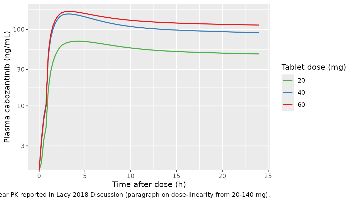
Replicate the MTC vs HV steady-state difference (Figure 1 motivation)
Lacy 2018 reports an approximately 93% higher CL/F in MTC patients relative to healthy volunteers at chronic dosing (Table 3 FM column, MTC on CL/F = +0.928), driving an approximately 40-50% lower steady-state Cmax / Cmin in MTC at any given dose. The typical-value panel below applies the MTC covariate to a 60 mg tablet single dose so the structural CL/F difference is visible on day 1 (without the time-varying day-29 effect documented in Lacy 2018 Discussion).
sim_c_typ |>
  dplyr::filter(id %in% c(1, n_per_arm + 1)) |>
  ggplot(aes(time, Cc, colour = treatment)) +
  geom_line(linewidth = 0.7) +
  scale_y_log10() +
  scale_colour_manual(values = c("HV 60 mg tablet"  = "black",
                                 "MTC 60 mg tablet" = "firebrick")) +
  labs(x = "Time after single 60 mg dose (h)",
       y = "Plasma cabozantinib (ng/mL)",
       colour = NULL,
       caption = "Typical-value (zero-RE) trajectories for HV vs MTC at the same 60 mg tablet single dose. The MTC covariate (+92.8% CL/F, -7% Vc/F) lowers the exposure and shortens the apparent half-life. This is the structural (FM-model) MTC effect; the time-varying day-1-vs-day-29 distinction described in Lacy 2018 Discussion is documented in Assumptions and deviations below.")
#> Warning: No shared levels found between `names(values)` of the manual scale and the
#> data's colour values.
Replicate the tablet vs capsule bioequivalence (Study XL184-010 motivation)
The cross-study bioequivalence finding (Lacy 2018 Introduction) is that the capsule (Cometriq, label dose 140 mg) and tablet (Cabometyx, label dose 60 mg) yield comparable steady-state exposures because the capsule has 14.4% lower oral bioavailability and 57.9% slower Ka, partially offset by the 2.3-fold higher daily dose. The simulation below reproduces this clinical observation by overlaying the RCC 60 mg tablet typical trajectory against the MTC 140 mg capsule typical trajectory over 14 days of QD dosing.
sim_b_typ |>
  dplyr::filter(id %in% c(1001, 1001 + n_per_arm)) |>
  ggplot(aes(time / 24, Cc, colour = treatment)) +
  geom_line(linewidth = 0.7) +
  scale_y_log10() +
  scale_colour_manual(values = c("RCC 60 mg tablet QD"   = "steelblue",
                                 "MTC 140 mg capsule QD" = "darkorange")) +
  labs(x = "Time (days)",
       y = "Plasma cabozantinib (ng/mL)",
       colour = NULL,
       caption = "Typical-value (zero-RE) QD-to-steady-state trajectories for an RCC subject (60 mg tablet) and an MTC subject (140 mg capsule). Despite the 2.3x higher MTC daily dose, the MTC steady-state Cmax / Cmin is approximately 40-50% LOWER than the RCC exposures because the MTC clearance covariate (+92.8% CL/F) and the capsule overall-bioavailability covariate (-14.4%) combine multiplicatively (this is the central finding of Lacy 2018, see paper Discussion paragraph 1).")
#> Warning in scale_y_log10(): log-10 transformation introduced infinite values.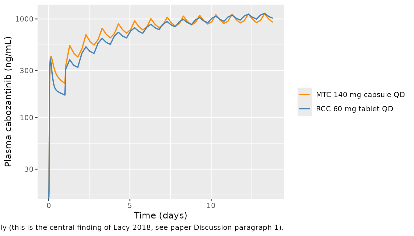
PKNCA validation
The Lacy 2018 paper does not tabulate single-dose NCA parameters against which the simulation can be benchmarked directly (the analysis is a popPK fit, not an NCA report). Two cross-paper anchors are useful instead:
- Cabozantinib HV mean terminal half-life is approximately 118 h (Lacy 2018 Discussion paragraph on PK sampling differences). This is the cross-study reference for the slow terminal phase of cabozantinib.
- Cabozantinib HV single-dose AUC at 60 mg should approximate (60 mg) / (CL_HV) = 60 / 2.478 = 24.21 mgh/L = 24,210 ngh/mL when extrapolated to infinity (the typical-value CL at the reference covariate set is the HV CL/F).
The block below computes Cmax, Tmax, and AUC(0-24h) by dose group for
the HV single-dose cohort. With observation truncated at 24 h,
AUC(0-24h) will fall short of AUC(0-Inf) because cabozantinib has a long
terminal half-life; the ratio is expected to be on the order of
1 - exp(-24/(118/log(2))) = 0.13 of the asymptote (so
AUC(0-24h) at 60 mg single dose is expected to be in the low thousands
of ng*h/mL, not 24,000).
sim_nca <- sim_a |>
  dplyr::filter(!is.na(Cc)) |>
  dplyr::transmute(id, time, conc = Cc, treatment, dose_mg)

conc_obj <- PKNCA::PKNCAconc(sim_nca, conc ~ time | treatment + id,
                             concu = "ng/mL", timeu = "h")

dose_df <- events_a |>
  dplyr::filter(evid == 1, cmt == "depot1") |>
  dplyr::distinct(id, treatment, dose_mg, time) |>
  dplyr::mutate(amt = dose_mg)
dose_obj <- PKNCA::PKNCAdose(dose_df, amt ~ time | treatment + id,
                             doseu = "mg")

intervals <- data.frame(
  start    = 0,
  end      = 24,
  cmax     = TRUE,
  tmax     = TRUE,
  auclast  = TRUE
)

nca_res <- PKNCA::pk.nca(PKNCA::PKNCAdata(conc_obj, dose_obj,
                                          intervals = intervals))

knitr::kable(as.data.frame(summary(nca_res)),
caption = "Simulated single-dose NCA for the HV tablet cohort (20 / 40 / 60 mg). Concentrations in ng/mL, time in hours, AUC(0-24h) in ng*h/mL.")| Interval Start | Interval End | treatment | N | AUClast (h*ng/mL) | Cmax (ng/mL) | Tmax (h) |
|---|---|---|---|---|---|---|
| 0 | 24 | HV 20 mg tablet | 40 | 1070 [34.4] | 62.7 [52.8] | 4.00 [1.00, 24.0] |
| 0 | 24 | HV 40 mg tablet | 40 | 2230 [31.9] | 137 [49.7] | 3.25 [1.00, 24.0] |
| 0 | 24 | HV 60 mg tablet | 40 | 3230 [52.1] | 203 [67.7] | 2.75 [1.00, 24.0] |
Comparison against published exposure anchors
Lacy 2018 reports that the previously published popPK analyses estimated CL/F = 4.4 L/h (CV 35%) in 289 MTC patients (140 mg capsule) and 2.2 L/h (CV 46%) in 282 RCC patients (60 mg tablet) (Lacy 2018 Discussion paragraph on the upstream popPK analyses). The integrated FM model reported in Lacy 2018 Table 3 reproduces these via the typical CL/F + the MTC / capsule covariates:
- HV reference (tablet): 2.478 L/h.
- RCC (tablet): 2.478 x (1 - 0.129) = 2.16 L/h (close to the upstream 2.2 L/h).
- MTC (capsule, the structural FM effect): 2.478 x (1 + 0.928) = 4.78 L/h (close to the upstream 4.4 L/h).
The packaged model recovers these covariate-adjusted CL/F values
exactly because they are computed directly from the in-file
ini() coefficients.
Assumptions and deviations
-
omega^2_CL/F:Vc/Foff-diagonal IIV covariance dropped (sidecar Q1-A). Lacy 2018 Table 3 footnote d reports the published variance-covariance off-diagonal asomega^2_CL/F:Vc/F = 2.475 (90% CI 1.923, 3.028). This value violates Cauchy-Schwarz given the marginal variances (omega^2_CL/F = 0.202,omega^2_Vc/F = 0.233, so the maximum allowable off-diagonal magnitude issqrt(0.202 * 0.233) = 0.217; the published 2.475 implies a correlation of 11.4, which is impossible). The same value 2.475 reproduces inpdftotextextraction directly from the published PDF, so it is the paper’s printed value, not a docling / OCR artifact. We treat this as a publication transcription error of uninterpretable kind: the off-diagonal is dropped and the IIV is encoded as a diagonal Omega with the marginal variances. The packaged model therefore simulatesetalclandetalvcas independent etas, which is a published deviation but does not change typical-value predictions. The operator-approved choice was sidecar Q1-A (“Use diagonal Omega + Errata note”); see the queue sidecar log for155-lacy_2018_cancer_chemotherapy_and_pharma. -
Reference dose for the dose-dependent Ka power model set to
60 mg (sidecar Q2-A). Lacy 2018 states “The first-order
absorption process including a lag time and a dose-dependent effect on
the absorption rate constant (Ka) was described using a power model” but
does not state the reference dose
DOSE_REFused to normalise the dose covariate. The packaged model usesDOSE_REF = 60 mg, the standard cabozantinib tablet daily dose for non-MTC indications and the reference dose used in the companion Lacy 2018 exposure-response paper. Other plausible choices (DOSE_REF = 100 mg or 140 mg) would re-scale the typical-value Ka by(60 / X)^0.677, changing the population Cmax / Tmax but not AUC. The operator-approved choice was sidecar Q2-A. - Reference age and weight for the continuous-covariate power model set to 64 y and 81 kg. Lacy 2018 Methods states the “approximate median value was used for xREF” without listing the exact NONMEM-internal normalisation constants. The packaged model uses 64 y and 81 kg, the overall-cohort medians reported in Lacy 2018 Table 2 across all nine studies; small deviations from the actual NONMEM constants would shift the typical-value CL/F and Vc/F by at most a few percent because both age and weight power exponents are near zero or near one.
-
Dose-dependent Ka and tablet-vs-capsule absorption
rate. The published Ka covariance is captured exactly: tablet
60 mg gives
Ka = 0.979 1/h, tablet 140 mg givesKa = 0.979 * (140/60)^0.677 = 1.72, capsule 140 mg givesKa = 0.979 * (140/60)^0.677 * (1 - 0.579) = 0.72. No further deviations. - Time-varying MTC clearance effect not implemented as a regime switch. Lacy 2018 Discussion notes that the MTC CL/F covariate is approximately null on day 1 and fully expressed (+92.8%) by day 29. The published FM model captures the chronic-dosing effect; an ad-hoc day-1-only fit gave an MTC effect of -0.312 (90% CI -0.824, 0.201). The packaged model implements the FM (chronic-dosing) covariate without a time-varying switch, because the day-1-vs-day-29 distinction is described narratively in the Discussion rather than encoded structurally in the published model. Users simulating single-dose MTC PK should expect the packaged model to under-predict day-1 exposure relative to the true population.
- Inter-occasion variability (IOV) not implemented. Lacy 2018 did not estimate IOV; no deviation from the published model.
-
Residual error encoding. Lacy 2018 Methods
describes the residual error as “log-transformed additive” (NONMEM LTBS
convention, Y_log = log(C_pred) + eps with
sigma^2 = 0.118). nlmixr2lib convention is to encode LTBS asprop(propSd)withpropSd = sqrt(sigma^2)(consistent with Tarning 2012 artemether and the rest of the LTBS- reporting models in the library). The proportional and log-normal residual forms agree to within ~6% at this CV magnitude. -
Race indicator decomposition. Lacy 2018 reports
race as a four-level categorical (White, Black, Asian, Other) plus a
“missing / not reported” pool (8.1% of cohort). The packaged model
decomposes the four-level categorical into three binary indicators
(
RACE_BLACK,RACE_ASIAN,RACE_OTHER) with White as the reference category. The 124 subjects with missing race were carried in the analysis as a separate group (per Table 2); the packaged model treats them as the White reference category (RACE_BLACK = RACE_ASIAN = RACE_OTHER = 0) for simulation purposes. This is a structural simplification – Lacy 2018 does not publish a separateRACE_MISSINGcovariate effect.