Tigecycline (Borsuk-De Moor 2018)
Source:vignettes/articles/BorsukDeMoor_2018_tigecycline.Rmd
BorsukDeMoor_2018_tigecycline.RmdModel and source
- Citation: Borsuk-De Moor A, Rypulak E, Potrec B, Piwowarczyk P, Borys M, Sysiak J, Onichimowski D, Raszewski G, Czuczwar M, Wiczling P. Population pharmacokinetics of high-dose tigecycline in patients with sepsis or septic shock. Antimicrob Agents Chemother. 2018;62(4):e02273-17. doi:10.1128/AAC.02273-17. Structural model, parameter estimates and the random-effects structure are taken from Borsuk-De Moor 2018 Table 2 and the ‘Pharmacokinetic modeling’ subsection of Materials and Methods. The article’s supplemental material (AAC.02273-17_zac004187006s1.pdf) contains only the chromatographic method, its validation, and Figures S1-S6 (time-dependent covariate summaries, goodness-of-fit, individual fits and eta-versus-covariate scatter plots); it carries no NONMEM control stream and no additional parameter values.
- Description: Two-compartment linear IV population PK model for high-dose tigecycline in adult ICU patients with sepsis or septic shock. Carries interindividual variability on clearance and on both volumes, plus interoccasion variability on clearance and peripheral volume across up to eight 12-hourly dosing occasions, and a combined additive-plus-proportional residual error. No covariate was retained: a visual search over age, weight, height, sex, ECMO, CRRT, dialysis volume, ultrafiltration rate, extravascular lung water index, cardiac output, SOFA score and procalcitonin found no systematic relationship with the individual PK parameters. Fitted by NONMEM 7.3 FOCE-I with eta-epsilon interaction (ADVAN3 TRANS4) to 940 plasma concentrations from 37 patients receiving a 200 mg loading dose followed by 100 mg every 12 h as 30-minute infusions.
- Article: https://doi.org/10.1128/AAC.02273-17
This is the third tigecycline model in the library fitted to a
critically ill cohort, and the only one of the four fitted to the
high-dose regimen. The licensed regimen is a 100 mg loading
dose followed by 50 mg every 12 h; Luo_2023_tigecycline,
Song_2024_tigecycline and Su_2024_tigecycline
were all fitted on that schedule. Borsuk-De Moor 2018 doubles it
throughout - 200 mg loading, then 100 mg every 12 h - following the
Ramirez 2013 and De Pascale 2014 findings that the licensed dose
underexposes ICU patients.
Two features distinguish it structurally from its siblings:
- Interoccasion variability. Samples were drawn after every dose, so the authors could split within-patient from between-patient variability. Doing so moved a substantial share of clearance variability out of IIV: the remaining IIV on CL is 17.3%, roughly half of what comparable studies report, with a further 14.4% carried as IOV.
- No retained covariate. Twelve covariates were screened - including the weight, creatinine clearance and sex terms that Van Wart 2006 and Rubino 2010 retained - and none showed a systematic relationship. The paper’s conclusion is that uniform dosing is sufficient in this population and that adjustment should be driven by the pathogen MIC instead.
Population
Thirty-seven adults with sepsis or septic shock in two Polish tertiary medical/surgical ICUs (Lublin and Olsztyn), contributing 940 analysed plasma tigecycline concentrations from 942 collected (two removed as CWRES > 5 outliers). Median age 61 years (range 25-79), weight 80 kg (50-129), height 175 cm (158-190); 11 of 37 (29.7%) were female. The cohort was severely ill: median SOFA score 13 points (range 2.0-21), median albumin 2.2 g/dL (1.5-3.6), median procalcitonin 8.22 ug/L (0.16-122), and 23 of 37 patients died. Thirty of 37 were on continuous renal replacement therapy and 2 on ECMO.
Every patient received the same high-dose regimen: a 200 mg loading dose as a 30-minute intravenous infusion, then 100 mg every 12 h as 30-minute infusions, for 2 to 8 doses over 1 to 4 consecutive days. Arterial blood was sampled at 0.5, 2, 4, 8 and 12 h after every dose - the dense per-occasion schedule that makes the IOV estimable.
The same information is available programmatically via
readModelDb("BorsukDeMoor_2018_tigecycline")()$population.
Source trace
Every ini() entry in
inst/modeldb/specificDrugs/BorsukDeMoor_2018_tigecycline.R
carries an in-file comment naming its origin. They are collected here
for review. All values come from the main article; the supplemental
material (AAC.02273-17_zac004187006s1.pdf) contains only
the chromatographic method, its validation, and Figures S1-S6, and
carries no NONMEM control stream and no additional parameter values.
| Equation / parameter | Value | Source location |
|---|---|---|
| Two-compartment linear disposition, clearance/volume parameterisation | ADVAN3 TRANS4 |
Materials and Methods, Pharmacokinetic modeling: “a two-compartment model was used”; “parametrized in terms of clearances (CL and Q) and volumes of distribution (V1 and V2)” |
lcl = log(CL) |
22.1 L/h | Table 2, theta CL (RSE 3.16%; bootstrap 22.1, 90% CI
20.9-23.2) |
lvc = log(V1) |
162 L | Table 2, theta V1 (RSE 5.3%; bootstrap 163, 90% CI
150-176) |
lq = log(Q) |
69.4 L/h | Table 2, theta Q (RSE 32.6%; bootstrap 67.3, 90% CI
41.9-98.4) |
lvp = log(V2) |
87.9 L | Table 2, theta V2 (RSE 8.67%; bootstrap 87.6, 90% CI
76.1-101) |
IIV form P = theta * exp(eta) * exp(kappa)
|
log-normal | Materials and Methods: “P(i,k) = theta_P exp(eta_P,i) exp(kappa_P,i,k)” |
etalcl |
17.3 % CV -> 0.029929 | Table 2, omega^2 CL (% CV) (RSE 19%, shrinkage
7.3%) |
etalvc |
19.2 % CV -> 0.036864 | Table 2, omega^2 V1 (% CV) (RSE 29.2%, shrinkage
6.7%) |
etalvp |
38.7 % CV -> 0.149769 | Table 2, omega^2 V2 (% CV) (RSE 40.8%, shrinkage
22.4%) |
| No IIV on Q | fixed at 0 | Table 2, omega^2 Q (% CV) = “0 FIX”; Results: “it was
not possible to estimate the interindividual variability (IIV) for the
intercompartmental clearance (Q2)” |
etaiov_lcl_1 .. etaiov_lcl_8
|
14.4 % CV -> 0.020736 | Table 2, pi^2 CL (% CV) (RSE 35%), with per-occasion
shrinkage printed for Occasions 1-8 |
etaiov_lvp_1 .. etaiov_lvp_8
|
20.8 % CV -> 0.043264 | Table 2, pi^2 V2 (% CV) (RSE 66.4%), with per-occasion
shrinkage printed for Occasions 1-8 |
| Occasion count = 8; shared magnitude across occasions | - | Table 2 prints Occasion 1-8 shrinkage rows; Materials and Methods: “The IIV and IOV variances were assumed to be constant across occasions” |
addSd |
0.0210 mg/L | Table 2, sigma_add (ug/ml); footnote a: “sigma_add,
additive residual random error” |
propSd |
13.0 % CV -> 0.130 | Table 2, sigma^2_prop (% CV); footnote a:
“sigma^2_prop, variance of proportional residual random error” |
| Combined additive + proportional residual | - | Materials and Methods: “modeled using a combined additional and proportional error model” |
| Dosing regimen simulated below | 200 mg then 7 x 100 mg q12h, 30-min infusions | Patients and study design; Figure 6 caption |
Published Vss
|
250 L | Discussion: “Mean Vss in our study is 250 liters” |
| Published accumulation ratio | 1.57 | Discussion: “accumulation ratio of 1.57 in our study compared to 4.00 [18] and 2.55 [19]” |
Virtual cohort
The cohort reproduces the study’s own regimen and its eight dosing
occasions. No covariate enters the model, so the only subject-level
column needed is the occasion indicator OCC, which is
time-varying: occasion k spans
[(k-1) * 12, k * 12) hours, matching the paper’s definition
of an occasion as one 12-hourly administration.
n_sub <- 150L
tau <- 12      # dosing interval (h)
t_inf <- 0.5   # infusion duration (h)
load_mg <- 200
maint_mg <- 100
n_doses <- 8L  # loading dose + 7 maintenance doses, per Figure 6
t_end <- as.numeric(n_doses) * tau

dose_times <- seq(0, by = tau, length.out = n_doses)
dose_amts <- c(load_mg, rep(maint_mg, n_doses - 1L))

# Occasion index for an arbitrary time, clamped to the eight modelled slots.
occ_of <- function(time) pmin(pmax(floor(time / tau) + 1L, 1L), 8L)

subj <- data.frame(id = seq_len(n_sub))

doses <- subj |>
  tidyr::crossing(dose_idx = seq_len(n_doses)) |>
  dplyr::mutate(
    time = dose_times[dose_idx],
    amt = dose_amts[dose_idx],
    evid = 1L,
    # Explicit infusion rate (mg/h). An IV dose given without a rate is
    # delivered as a bolus, which every AUC-based gate would still pass, so
    # the rate is set here rather than left to a duration column.
    rate = amt / t_inf,
    cmt = "central"
  ) |>
  dplyr::select(-dose_idx)

obs_times <- seq(0, t_end, by = 0.5)
obs <- subj |>
  tidyr::crossing(time = obs_times) |>
  dplyr::mutate(amt = NA_real_, evid = 0L, rate = NA_real_, cmt = "central")

events <- dplyr::bind_rows(doses, obs) |>
  dplyr::mutate(OCC = occ_of(time)) |>
  dplyr::arrange(id, time, dplyr::desc(evid)) |>
  as.data.frame()

# All eight occasion slots must actually be exercised, otherwise the IOV
# structure is only nominally tested.
stopifnot(
  setequal(unique(events$OCC), 1:8),
  dplyr::n_distinct(events$id) == n_sub,
  all(events$rate[events$evid == 1] == events$amt[events$evid == 1] / t_inf)
)
Simulation
# `readModelDb()` returns the model FUNCTION; `rxode()` turns it into the rxUi
# that carries `$simulationModel`, `$omega` and `$theta`.
mod <- rxode2::rxode(readModelDb("BorsukDeMoor_2018_tigecycline"))
#> ℹ parameter labels from comments will be replaced by 'label()'
#> Warning: some etas defaulted to non-mu referenced, possible parsing error: etaiov_lcl_1, etaiov_lcl_2, etaiov_lcl_3, etaiov_lcl_4, etaiov_lcl_5, etaiov_lcl_6, etaiov_lcl_7, etaiov_lcl_8, etaiov_lvp_1, etaiov_lvp_2, etaiov_lvp_3, etaiov_lvp_4, etaiov_lvp_5, etaiov_lvp_6, etaiov_lvp_7, etaiov_lvp_8
#> as a work-around try putting the mu-referenced expression on a simple line
stopifnot(inherits(mod, "rxUi"), !is.null(mod$simulationModel))
# 3 IIV etas + 2 parameters x 8 occasion slots of IOV.
stopifnot(identical(dim(mod$omega), c(19L, 19L)))

# `omega` is passed explicitly: rxode2 caches the previous solve's omega against
# the compiled model, so a later population solve can silently collapse onto one
# typical subject (and a later typical-value solve can silently re-sample etas).
sim <- rxode2::rxSolve(
  mod$simulationModel, events,
  omega = mod$omega, keep = "OCC"
) |>
  as.data.frame()

stopifnot(all(c("Cc", "sim", "cl", "vc", "q", "vp", "OCC") %in% names(sim)))
# Cc is exactly 0 at t = 0: the observation sits at the start of the first
# 30-minute infusion, before any drug has been delivered.
stopifnot(!anyNA(sim$Cc), all(sim$Cc >= 0))
stopifnot(all(sim$Cc[sim$time > 0] > 0))
stopifnot(all(sim$Cc[sim$time == 0] == 0))

# Guard the population direction of the omega-caching bug: IIV must have varied.
stopifnot(dplyr::n_distinct(round(sim$vc, 8)) > 1L)
# Guard the IOV direction: clearance must vary WITHIN a subject across
# occasions, which only IOV can produce (no covariate acts on CL).
within_subject_cl_levels <- sim |>
  dplyr::group_by(id) |>
  dplyr::summarise(n_cl = dplyr::n_distinct(round(cl, 8)), .groups = "drop")
stopifnot(all(within_subject_cl_levels$n_cl == 8L))
Replicate published figures
Figure 6 - typical-value concentration-time profile
Figure 6 of Borsuk-De Moor 2018 simulates tigecycline concentrations after the 200 mg loading dose and seven subsequent 100 mg doses at 12-hour intervals, using the typical population parameters (the black solid line of that figure; the red dashed lines are the three comparator models, which are not reproduced here).
mod_typ <- rxode2::zeroRe(mod)
#> Warning: some etas defaulted to non-mu referenced, possible parsing error: etaiov_lcl_1, etaiov_lcl_2, etaiov_lcl_3, etaiov_lcl_4, etaiov_lcl_5, etaiov_lcl_6, etaiov_lcl_7, etaiov_lcl_8, etaiov_lvp_1, etaiov_lvp_2, etaiov_lvp_3, etaiov_lvp_4, etaiov_lvp_5, etaiov_lvp_6, etaiov_lvp_7, etaiov_lvp_8
#> as a work-around try putting the mu-referenced expression on a simple line
typ_events <- events |> dplyr::filter(id == 1L)

# `omega = NA` is the only reliable way to force a typical-value solve;
# zeroRe() alone is not sufficient once a stochastic solve has run.
typ <- rxode2::rxSolve(mod_typ, typ_events, omega = NA, keep = "OCC") |>
  as.data.frame()

# If etas were silently re-sampled, cl would vary across occasions here too.
stopifnot(dplyr::n_distinct(round(typ$cl, 8)) == 1L)
stopifnot(dplyr::n_distinct(round(typ$vp, 8)) == 1L)

ggplot(typ, aes(time, Cc)) +
  geom_line() +
  geom_vline(xintercept = dose_times, linetype = "dotted", alpha = 0.4) +
  scale_y_log10() +
  labs(
    x = "Time (h)", y = "Tigecycline (mg/L)",
    title = "Typical-value profile, 200 mg then 7 x 100 mg q12h",
    caption = "Replicates the black solid line of Figure 6 of Borsuk-De Moor 2018."
  )
#> Warning in scale_y_log10(): log-10 transformation introduced infinite values.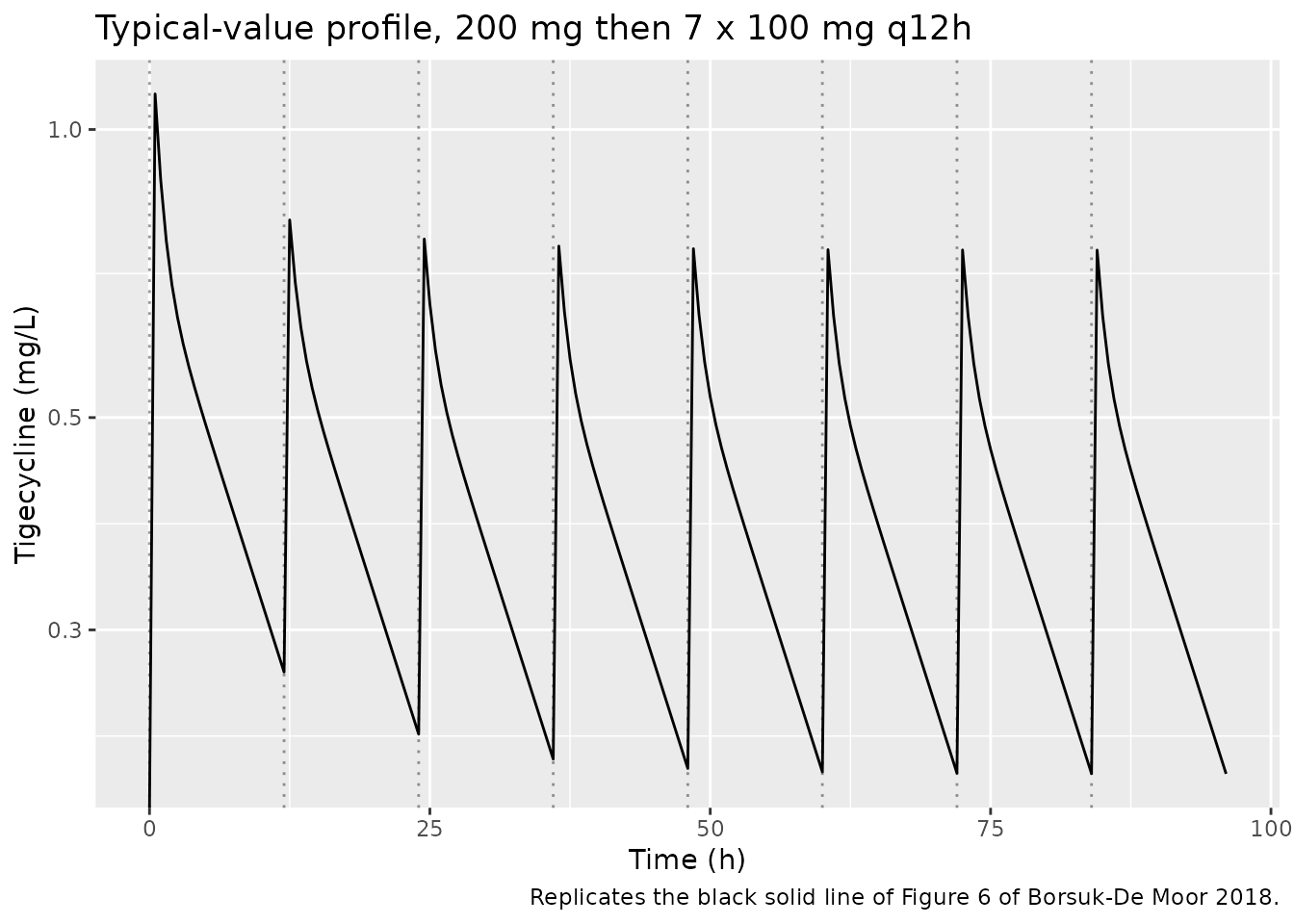
Figure 2 - visual predictive check
Figure 2 is a VPC over a dosing interval. The observed concentrations
behind it are not public, so only the simulated side is reproduced: the
5th, 50th and 95th percentiles of simulated observations
(sim, the individual prediction plus a combined
additive-and-proportional residual draw).
sim |>
  dplyr::group_by(time) |>
  dplyr::summarise(
    Q05 = quantile(sim, 0.05),
    Q50 = quantile(sim, 0.50),
    Q95 = quantile(sim, 0.95),
    .groups = "drop"
  ) |>
  ggplot(aes(time, Q50)) +
  geom_ribbon(aes(ymin = Q05, ymax = Q95), alpha = 0.25) +
  geom_line() +
  scale_y_log10() +
  labs(
    x = "Time (h)", y = "Tigecycline (mg/L)",
    title = "Simulated 5th / 50th / 95th percentiles over the 96 h course",
    caption = "Replicates the predicted percentiles of Figure 2 of Borsuk-De Moor 2018."
  )
#> Warning in transformation$transform(x): NaNs produced
#> Warning in scale_y_log10(): log-10 transformation introduced infinite values.
#> Warning: Removed 1 row containing missing values or values outside the scale range
#> (`geom_ribbon()`).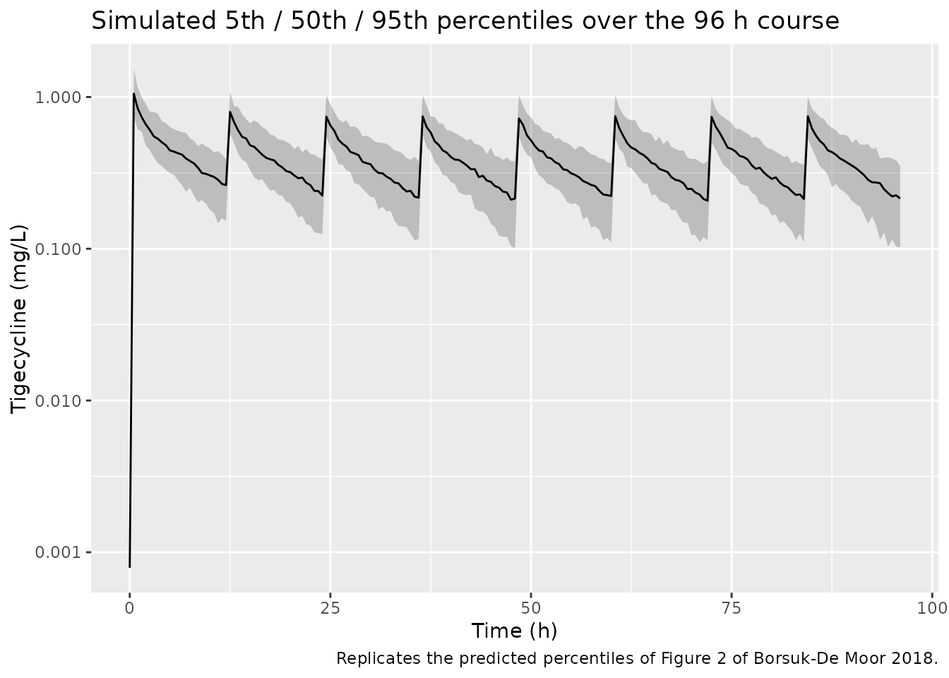
Structural validation
Closed-form biexponential
rxode2 recognises a cl / vc /
q / vp parameter set and replaces the written
ODE system with its analytic solution. That substitution is silent, and
when a q / vp pair is missing it
collapses a two-compartment model to one compartment while leaving every
AUC-based gate passing. The check below is therefore the load-bearing
structural test: the typical-value solve is compared against the
two-compartment infusion biexponential evaluated independently from the
ini() values.
Both sides use the same parameters, so the only difference is numerical integration error and the bound is tight.
theta <- mod$theta
cl_t <- exp(theta[["lcl"]])
vc_t <- exp(theta[["lvc"]])
q_t <- exp(theta[["lq"]])
vp_t <- exp(theta[["lvp"]])

k10 <- cl_t / vc_t
k12 <- q_t / vc_t
k21 <- q_t / vp_t

# Hybrid rate constants of the two-compartment system.
a_sum <- k10 + k12 + k21
b_prod <- k10 * k21
lam1 <- (a_sum + sqrt(a_sum^2 - 4 * b_prod)) / 2   # distribution
lam2 <- (a_sum - sqrt(a_sum^2 - 4 * b_prod)) / 2   # terminal
stopifnot(lam1 > lam2, lam2 > 0)

coefA <- (lam1 - k21) / (lam1 - lam2)
coefB <- (k21 - lam2) / (lam1 - lam2)

# Superposition of constant-rate infusions: contribution of one dose of `amt`
# infused over `t_inf` at `t0`, evaluated at absolute time `tt`.
inf_conc <- function(tt, t0, amt) {
  r0 <- amt / t_inf
  te <- pmax(tt - t0, 0)                 # time since infusion start
  tin <- pmin(te, t_inf)                 # time spent infusing so far
  toff <- pmax(te - t_inf, 0)            # time since infusion end
  (r0 / vc_t) * (
    (coefA / lam1) * (1 - exp(-lam1 * tin)) * exp(-lam1 * toff) +
      (coefB / lam2) * (1 - exp(-lam2 * tin)) * exp(-lam2 * toff)
  )
}

cf <- rowSums(vapply(
  seq_len(n_doses),
  function(i) inf_conc(typ$time, dose_times[i], dose_amts[i]),
  numeric(nrow(typ))
))

# Drop t = 0, where both sides are exactly 0 and a relative error is undefined.
keep <- typ$time > 0
stopifnot(sum(keep) > 100, all(cf[keep] > 0))
rel_err <- abs(typ$Cc[keep] - cf[keep]) / cf[keep]
stopifnot(all(is.finite(rel_err)), max(rel_err) < 1e-5)
# t = 0 must still agree exactly.
stopifnot(all(abs(typ$Cc[!keep] - cf[!keep]) < 1e-12))
data.frame(
  Quantity = c(
    "Distribution rate constant (1/h)", "Terminal rate constant (1/h)",
    "Distribution half-life (h)", "Terminal half-life (h)",
    "Max relative difference, solve vs closed form"
  ),
  Value = c(
    lam1, lam2, log(2) / lam1, log(2) / lam2, max(rel_err)
  )
) |>
  knitr::kable(
    digits = c(0, 6),
    caption = "Two-compartment hybrid constants and the closed-form agreement bound."
)| Quantity | Value |
|---|---|
| Distribution rate constant (1/h) | 1.269506 |
| Terminal rate constant (1/h) | 0.084842 |
| Distribution half-life (h) | 0.545998 |
| Terminal half-life (h) | 8.169817 |
| Max relative difference, solve vs closed form | 0.000001 |
Steady-state volume of distribution
The Discussion states Vss = 250 L, defined in Materials
and Methods as the sum of V1 and V2. This is
the only volume quantity the paper reports beyond the two Table 2
estimates, and it confirms both are read on the same scale.
The model gives Vss = 249.9 L against the published 250
L.
Accumulation ratio
The Discussion reports an accumulation ratio of 1.57 on this regimen,
contrasted with 4.00 for Van Wart 2006 and 2.55 for Rubino 2010, and
attributes the difference to this study’s much smaller peripheral
volume. The ratio follows from the terminal rate constant and the dosing
interval, R = 1 / (1 - exp(-lambda_z * tau)).
This is the strongest published gate available, because
lambda_z is a joint function of all four structural
parameters: mis-transcribing any one of CL,
V1, Q or V2 moves it.
Vss above, by contrast, would survive a swap of
V1 and V2.
The model gives an accumulation ratio of 1.566 against the published 1.57.
Simulated accumulation
The analytic ratio above is a terminal-phase identity. The simulated
profile gives the same quantity empirically, as the ratio of
AUC over the last dosing interval to AUC over
the first, for a 100 mg dose on both. This needs a maintenance-only
schedule, so the loading dose is dropped for this check alone.
maint_doses <- subj |>
  dplyr::filter(id == 1L) |>
  tidyr::crossing(time = dose_times) |>
  dplyr::mutate(
    amt = maint_mg, evid = 1L, rate = maint_mg / t_inf, cmt = "central"
  )
maint_obs <- subj |>
  dplyr::filter(id == 1L) |>
  tidyr::crossing(time = seq(0, t_end, by = 0.05)) |>
  dplyr::mutate(amt = NA_real_, evid = 0L, rate = NA_real_, cmt = "central")
maint_ev <- dplyr::bind_rows(maint_doses, maint_obs) |>
  dplyr::mutate(OCC = occ_of(time)) |>
  dplyr::arrange(time, dplyr::desc(evid)) |>
  as.data.frame()

maint <- rxode2::rxSolve(mod_typ, maint_ev, omega = NA) |> as.data.frame()

auc_window <- function(d, lo, hi) {
  w <- d[d$time >= lo & d$time <= hi, ]
  sum(diff(w$time) * (utils::head(w$Cc, -1) + utils::tail(w$Cc, -1)) / 2)
}
auc_first <- auc_window(maint, 0, tau)
auc_last <- auc_window(maint, t_end - tau, t_end)
accum_sim <- auc_last / auc_first

# Approaches but has not fully reached the terminal-phase asymptote after eight
# intervals, so it sits just below the analytic value.
stopifnot(accum_sim > 1.50, accum_sim < accum)
Simulated AUC accumulation over eight intervals is 1.545, against the analytic asymptote of 1.566 and the published 1.57.
PKNCA validation
NCA is run on the typical-value single-dose profile, which is where
the paper’s two published derived quantities (CL and
Vss) are directly recoverable, and on the stochastic
cohort, to give the steady-state exposure summary a user of this model
will want.
single_ev <- data.frame(
  id = 1L,
  time = c(0, seq(0, 240, by = 0.05)),
  amt = c(load_mg, rep(NA_real_, length(seq(0, 240, by = 0.05)))),
  evid = c(1L, rep(0L, length(seq(0, 240, by = 0.05)))),
  rate = c(load_mg / t_inf, rep(NA_real_, length(seq(0, 240, by = 0.05)))),
  cmt = "central",
  OCC = 1L
)
single <- rxode2::rxSolve(mod_typ, single_ev, omega = NA) |> as.data.frame()

# A one-subject solve returns no `id` column, so PKNCA's grouping key has to be
# added back explicitly.
stopifnot(!"id" %in% names(single))
single$id <- 1L

sc <- single |>
  dplyr::filter(!is.na(Cc)) |>
  dplyr::select(id, time, Cc) |>
  dplyr::distinct(id, time, .keep_all = TRUE) |>
  dplyr::arrange(id, time) |>
  as.data.frame()

conc_single <- PKNCA::PKNCAconc(sc, Cc ~ time | id)
dose_single <- PKNCA::PKNCAdose(
  data.frame(id = 1L, time = 0, amt = load_mg, duration = t_inf),
  amt ~ time | id, duration = "duration", route = "intravascular"
)

# The terminal phase of a two-compartment profile is only clean well after
# distribution is complete; an automatic lambda-z window would otherwise wander
# into the distribution phase and bias half-life (and therefore Vss).
iv_intervals <- data.frame(
  start = 0, end = Inf,
  aucinf.obs = TRUE, cl.obs = TRUE, vss.obs = TRUE,
  half.life = TRUE, mrt.iv.obs = TRUE,
  impute = NA_character_
)
nca_single <- PKNCA::pk.nca(PKNCA::PKNCAdata(
  conc_single, dose_single, intervals = iv_intervals
))
single_tbl <- as.data.frame(nca_single$result)
getp <- function(code) {
  v <- single_tbl$PPORRES[single_tbl$PPTESTCD == code]
  stopifnot(length(v) == 1L, is.finite(v))
  v
}

# Mass balance: for an IV dose, CL * AUCinf must return the dose exactly.
# This is a pure closed-form identity for a linear model, so the bound is tight.
stopifnot(abs(cl_t * getp("aucinf.obs") / load_mg - 1) < 1e-3)
# NCA half-life must recover the analytic terminal half-life.
stopifnot(abs(getp("half.life") - log(2) / lam2) < 0.05)
Comparison against the published derived parameters
Borsuk-De Moor 2018 publishes no NCA table - no Cmax, Tmax, AUC or
half-life is reported for the cohort - so the reference side below is
the paper’s two published derived quantities: the Table 2 clearance
estimate and the Discussion’s Vss. Recovering both from an
independent NCA of the simulated profile confirms that the model as
encoded reproduces the paper’s own summary of its fit.
One correction is needed first. PKNCA’s vss.obs is
defined as cl.obs * mrt.obs, which for an infusion does
not subtract the infusion-duration term; on this 30-minute
infusion it overstates Vss by CL * t_inf / 2 =
5.5 L, or 2.2%. The steady-state volume the paper reports is
V1 + V2, the infusion-corrected quantity, so the comparison
below uses cl.obs * mrt.iv.obs instead.
reference_nca <- data.frame(
  cl.obs = 22.1,   # Borsuk-De Moor 2018 Table 2, theta CL
  vss.obs = 250    # Borsuk-De Moor 2018 Discussion, "Mean Vss in our study is 250 liters"
)

# PKNCA's `vss.obs` is `cl.obs * mrt.obs`, WITHOUT the infusion-duration
# correction - assert that definition rather than assume it.
stopifnot(abs(getp("vss.obs") - getp("cl.obs") * getp("mrt.obs")) < 1e-6)

# For a 30-minute infusion the uncorrected form overstates Vss by
# CL * t_inf / 2 = 5.5 L. The paper's Vss is V1 + V2, the corrected quantity,
# so the comparison uses `mrt.iv.obs`, which PKNCA reports separately and which
# does carry the correction.
simulated_nca <- data.frame(
  cl.obs = getp("cl.obs"),
  vss.obs = getp("cl.obs") * getp("mrt.iv.obs")
)

nca_cmp <- nlmixr2lib::ncaComparisonTable(
  simulated = simulated_nca,
  reference = reference_nca,
  params = c("cl.obs", "vss.obs"),
  units = c(cl.obs = "L/h", vss.obs = "L")
)
knitr::kable(
  nca_cmp,
  digits = 2,
  caption = paste(
    "Simulated NCA of the typical-value 200 mg profile against the derived",
    "parameters published by Borsuk-De Moor 2018."
  )
)| NCA parameter | Reference | Simulated | % diff |
|---|---|---|---|
| CL/F (L/h) | 22.1 | 22.1 | +0.0% |
| Vss/F (L) | 250 | 250 | -0.0% |
# `% diff` is a formatted DISPLAY string ("+0.0%", with a trailing "*" when the
# tolerance is exceeded), so it must be parsed rather than coerced: as.numeric()
# on it returns NA, and `all(NA < 1)` is NA, which would fail loudly here but
# pass vacuously under any assertion wrapped in isTRUE() or any().
pct <- as.numeric(sub("%$", "", sub("\\*$", "", nca_cmp[["% diff"]])))
stopifnot(length(pct) == 2L, !anyNA(pct))

# Both published quantities must be recovered, not merely be close.
stopifnot(all(abs(pct) < 1))
# No row may carry the >20% tolerance flag.
stopifnot(!any(grepl("*", nca_cmp[["% diff"]], fixed = TRUE)))Steady-state exposure across the cohort
sim_nca <- sim |>
  dplyr::filter(!is.na(Cc), time >= t_end - tau) |>
  dplyr::mutate(time = time - (t_end - tau)) |>
  dplyr::select(id, time, Cc) |>
  dplyr::distinct(id, time, .keep_all = TRUE) |>
  dplyr::arrange(id, time) |>
  as.data.frame()

# A time = 0 row is present by construction here (the grid lands on 84 h);
# the defensive bind is a no-op rather than an imputation.
stopifnot(all(sim_nca$time[!duplicated(sim_nca$id)] == 0))

conc_ss <- PKNCA::PKNCAconc(sim_nca, Cc ~ time | id)
dose_ss <- PKNCA::PKNCAdose(
  data.frame(id = seq_len(n_sub), time = 0, amt = maint_mg, duration = t_inf),
  amt ~ time | id, duration = "duration", route = "intravascular"
)
ss_intervals <- data.frame(
  start = 0, end = tau,
  cmax = TRUE, cmin = TRUE, cav = TRUE, tmax = TRUE, auclast = TRUE
)
nca_ss <- PKNCA::pk.nca(PKNCA::PKNCAdata(
  conc_ss, dose_ss, intervals = ss_intervals
))
ss_tbl <- as.data.frame(nca_ss$result)
ss_tbl |>
  dplyr::filter(PPTESTCD %in% c("cmax", "cmin", "cav", "tmax", "auclast")) |>
  dplyr::group_by(PPTESTCD) |>
  dplyr::summarise(
    median = median(PPORRES),
    p05 = quantile(PPORRES, 0.05),
    p95 = quantile(PPORRES, 0.95),
    .groups = "drop"
  ) |>
  dplyr::rename(
    "Parameter" = PPTESTCD, "Median" = median,
    "5th pctile" = p05, "95th pctile" = p95
  ) |>
  knitr::kable(
    digits = 2,
    caption = paste(
      "Simulated steady-state NCA over the eighth 12 h dosing interval, n = 150.",
      "Cmax / Cmin / Cav in mg/L, AUC0-12 in mg*h/L, Tmax in h.",
      "Borsuk-De Moor 2018 publishes no NCA table to compare against."
    )
)| Parameter | Median | 5th pctile | 95th pctile |
|---|---|---|---|
| auclast | 4.48 | 3.13 | 6.11 |
| cav | 0.37 | 0.26 | 0.51 |
| cmax | 0.75 | 0.61 | 0.93 |
| cmin | 0.20 | 0.10 | 0.34 |
| tmax | 0.50 | 0.50 | 0.50 |
cav <- ss_tbl$PPORRES[ss_tbl$PPTESTCD == "cav"]
auc <- ss_tbl$PPORRES[ss_tbl$PPTESTCD == "auclast"]
stopifnot(length(cav) == n_sub, !anyNA(cav))

# At steady state on a linear model, AUC0-tau = Dose / CL. Assert on the CENTRE
# of the cohort rather than on its extremes: the per-subject ratio varies with
# each subject's own drawn clearance, and the extreme of a random cohort is not
# reproducible across rxode2 builds.
ratio <- auc * (cl_t / maint_mg)
stopifnot(abs(median(ratio) - 1) < 0.10)
stopifnot(quantile(abs(ratio - 1), 0.9) < 0.40)
Interoccasion variability
IOV is what separates this model from its three tigecycline siblings,
so it is worth showing that it is actually active. For each subject,
clearance takes a different value on each of the eight occasions while
the subject’s own eta stays fixed; the spread
within a subject is the IOV, and its magnitude should match the
14.4% CV of Table 2.
iov_cv <- sim |>
  dplyr::group_by(id, OCC) |>
  dplyr::summarise(cl = dplyr::first(cl), .groups = "drop") |>
  dplyr::group_by(id) |>
  # Within-subject SD of log(CL) across occasions estimates the IOV omega.
  dplyr::summarise(sd_log_cl = sd(log(cl)), .groups = "drop")

# The within-subject SD of log(CL) across 8 occasions has a wide sampling
# distribution at n = 8, so assert on the cohort median against the published
# 0.144, not on any subject's own value.
stopifnot(abs(median(iov_cv$sd_log_cl) - 0.144) < 0.04)
sim |>
  dplyr::filter(id <= 12L) |>
  dplyr::group_by(id, OCC) |>
  dplyr::summarise(cl = dplyr::first(cl), .groups = "drop") |>
  ggplot(aes(factor(OCC), cl, group = id)) +
  geom_line(alpha = 0.6) +
  geom_point(size = 1) +
  geom_hline(yintercept = cl_t, linetype = "dashed") +
  labs(
    x = "Occasion", y = "Clearance (L/h)",
    title = "Interoccasion variability in clearance, first 12 subjects",
    caption = paste(
      "Each line is one subject across the eight dosing occasions.",
      "Dashed line is the typical value, 22.1 L/h."
    )
  )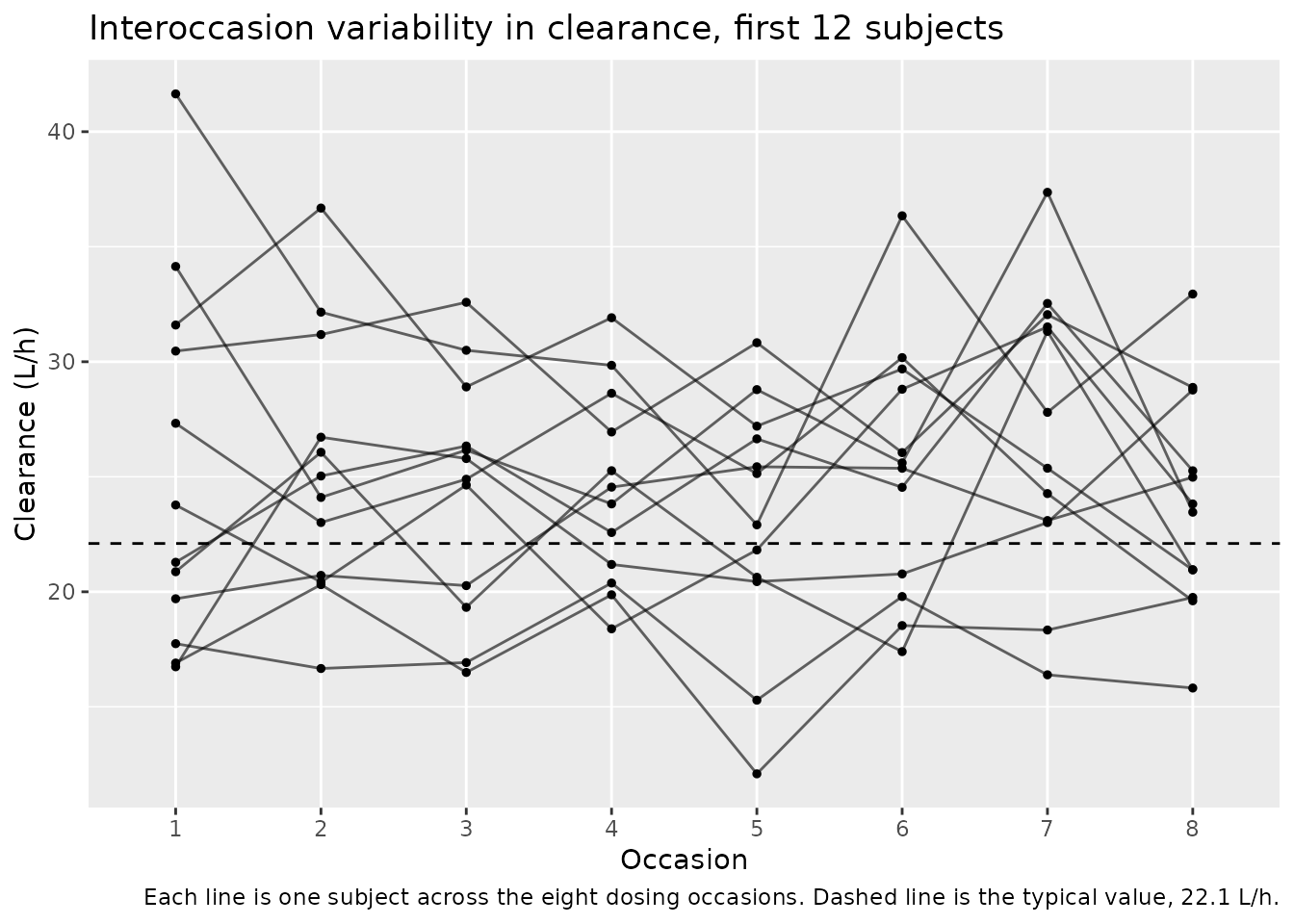
Median within-subject SD of log(CL) across occasions is 0.135, against the published IOV of 0.144 (14.4% CV, Table 2).
Assumptions and deviations
-
Omega scale (% CV reading). Table 2 labels its
variability rows
omega^2 CL (% CV),pi^2 CL (% CV)and so on - the estimated NONMEM variance displayed on a percent-CV scale - but gives no footnote stating the conversion formula. The conventional NONMEM readingCV% = 100 * sqrt(omega^2)is used, so each variance inini()is the printed percentage squared. The exact log-normal alternative,CV% = 100 * sqrt(exp(omega^2) - 1), would give 0.02949 / 0.03625 / 0.13966 for the three IIV terms instead of 0.02993 / 0.03686 / 0.14977 - a difference of at most 3.6% on the omega scale, largest for theV2term where the CV is largest. No published quantity discriminates the two readings: the bootstrap CIs are reported on the same % CV scale, and the RSE column is consistent with either. -
sigma_addandsigma^2_propare on different scales. Table 2’s footnote a names the additive row as the “additive residual random error” in ug/mL and the proportional row as the “variance of proportional residual random error”. The additive value is therefore used as printed (0.0210 mg/L, a standard deviation), while the proportional row is treated like the omegas (13.0% CV -> 0.130). This asymmetry is the paper’s, not an assumption. -
sigma_addRSE is internally inconsistent. Table 2 prints an RSE of 0.41% for the additive residual error, but its bootstrap 90% CI spans 0.000209-0.0357 around a median of 0.0224, a width implying an RSE near 100%. The point estimate is used regardless; the RSE is not used by the model. -
No IIV on Q. Table 2 prints
omega^2 Q (% CV)as “0 FIX” and the Results state the IIV on intercompartmental clearance was not estimable. Rather than encoding a zero-variance eta - which makes the omega matrix singular and breaks simulation -qsimply carries no eta. The two are mathematically equivalent. -
Occasion count and definition. Table 2 prints
per-occasion shrinkage for Occasions 1 through 8 and the study
administered 2 to 8 doses per patient, so eight occasion slots are
encoded with one 12-hourly dose per occasion. The paper states the IOV
variances “were assumed to be constant across occasions”, so occasions
2-8 are
fixed()at the occasion-1 value - the nlmixr2 spelling of NONMEM$OMEGA BLOCK(1) SAME. SettingOCC = 0disables IOV entirely. -
No covariates are encoded. Twelve covariates were
screened (age, weight, height, sex, ECMO, CRRT, dialysis volume,
ultrafiltration rate, ELWI, cardiac output, SOFA score, procalcitonin)
plus the derived body surface area and body mass index. The search was
visual - eta and kappa estimates plotted against covariates in
Figures 3, 4 and S4-S6 - and because no trend appeared, “formal
statistical testing was not employed”. No effect size exists to encode
for any of them. They are recorded in the model file’s
covariatesDataExcludedlist so the provenance of the screen survives, and they carry no convention warning because they are never referenced inmodel(). -
Procalcitonin units in Table 1. Table 1 prints
procalcitonin as “umol/liter” with a median of 8.22 and range 0.16-122.
Procalcitonin is a 13 kDa peptide reported clinically in ng/mL (= ug/L),
on which 8.22 is a typical septic value; 8.22 umol/L would be roughly
eight orders of magnitude above any reported concentration. The
covariatesDataExcludedentry records ug/L. This affects documentation only - the covariate is not in the model. - Cardiac output units in Table 1. Table 1 prints cardiac output in “liters”, a volume, with a median of 7.49 and range 2.55-15.8. Cardiac output is a flow; the quoted values match the L/min scale expected in a hyperdynamic septic cohort. Documentation only, as above.
-
Infusion rate is set explicitly in the event table.
Doses carry
rate = amt / 0.5rather than relying on a duration column, because an IV dose supplied without a rate is delivered as a bolus - and every AUC-based gate passes identically either way, so the error would be invisible. The closed-form check above compares against the infusion solution specifically. -
Vss is a weak gate; the accumulation ratio is the strong
one.
Vss= 250 L is justV1 + V2and would survive swapping the two volumes. The accumulation ratio of 1.57 depends on the terminal rate constant, which is a joint function of all four structural parameters, and is reproduced to 1.566. - The VPC panel shows the simulated side only. The observed concentrations behind Figure 2 are not published, so the figure reproduced here is the prediction band alone, not the observed-versus-predicted overlay.
-
Supplemental material adds nothing to the model.
The article’s supplement (
AAC.02273-17_zac004187006s1.pdf, retrieved from Europe PMC) contains the chromatographic method, its validation, and Figures S1-S6 - time-dependent covariate summaries, goodness-of-fit plots, individual fits, and eta-versus- covariate scatter plots. It carries no NONMEM control stream and no parameter values beyond those in Table 2.