Tacrolimus (Chen 2020b)
Source:vignettes/articles/Chen_2020b_tacrolimus.Rmd
Chen_2020b_tacrolimus.RmdModel and source
- Citation: Chen X, Wang DD, Xu H, Li ZP. Population pharmacokinetics and pharmacogenomics of tacrolimus in Chinese children receiving a liver transplant: initial dose recommendation. Transl Pediatr. 2020;9(5):576-586. doi:10.21037/tp-20-84
- Description: One-compartment population PK model with first-order absorption and first-order elimination for oral tacrolimus whole-blood concentrations in Chinese children after liver transplantation (Chen 2020). The absorption rate constant ka is fixed at 4.48 1/h from earlier paediatric liver-transplant tacrolimus models. Apparent oral clearance CL/F is allometrically scaled by body weight (fixed exponent 0.75, reference 70 kg), multiplied by 1.61 in recipients carrying a CYP3A5*1 allele (expressers) and reduced by 10.8% on concomitant Wuzhi capsule (Schisandra sphenanthera extract). Apparent volume V/F scales linearly with body weight (fixed exponent 1). Exponential IIV on V/F only; combined proportional-plus-additive residual error.
- Article: https://doi.org/10.21037/tp-20-84 (open access, PMC7658763)
Chen et al. (2020) combined routine therapeutic-drug-monitoring tacrolimus concentrations with next-generation pharmacogene sequencing in Chinese children after liver transplantation, fitted a one-compartment model with first-order absorption in NONMEM (FOCE-I), and used Monte Carlo simulation to recommend weight-banded initial doses for four genotype-by-co-medication groups. The final model (Results, Eqs. 7-8) is
- CL/F (L/h) = 6.57 x (WT/70)^0.75 x 1.61^CYP3A5 x (1 - 0.108 x WZ)
- V/F (L) = 77.6 x (WT/70)
- Ka = 4.48 1/h (fixed)
where CYP3A5 = 1 for a recipient carrying a CYP3A5*1 allele and WZ = 1 for concomitant Wuzhi capsule (a Schisandra sphenanthera extract that inhibits CYP3A).
Population
Twelve Chinese paediatric liver-transplant recipients (8 boys, 4 girls) treated at the Children’s Hospital of Fudan University between September 2014 and October 2019 (Table 1): age median 2.42 (range 0.47-7.96) years, weight median 13.00 (6.40-28.00) kg, post-transplantation day median 121 (4-1,877). Co-medications: glucocorticoid 11, aspirin 9, Wuzhi capsule 6, fluconazole 2. Recipient CYP3A5 genotype (Table 2): *1/*1 2, *1/*3 5, *3/*3 5. Whole-blood tacrolimus was measured by the Emit 2000 assay (2.0-30 ng/mL). The paper does not report the number of concentrations or their sampling times.
Source trace
| Element | Value | Source |
|---|---|---|
| Structure: 1-compartment, first-order absorption and elimination | – | Methods, Population pharmacokinetic model |
lka |
4.48 1/h (fixed) | Table 3; Methods (refs 23, 25) |
lcl |
6.57 L/h | Table 3; Eq. 7 |
lvc |
77.6 L | Table 3; Eq. 8 |
e_wt_cl |
0.75 (fixed), reference 70 kg | Methods Eq. 3 |
e_wt_vc |
1 (fixed), reference 70 kg | Methods Eq. 3; Eq. 8 |
e_cyp3a5_expr_cl |
1.61, form theta^CYP3A5
|
Table 3; Methods Eq. 4; Eq. 7 |
e_conmed_wuzhi_cl |
-0.108, form (1 + theta * WZ)
|
Table 3; Methods Eq. 6; Eq. 7 |
Exponential IIV P = TV * exp(eta)
|
– | Methods Eq. 1 |
etalvc |
0.396^2 = 0.156816 | Table 3 (omega V/F = 0.396, read as SD; see Assumptions) |
Residual error C = Cpre * (1 + eps1) + eps2
|
– | Methods Eq. 2 |
propSd |
0.288 | Table 3 (sigma 1, proportional) |
addSd |
0.720 ng/mL | Table 3 (sigma 2, additive) |
| CYP3A5 / WZ coding | CYP3A5*3/*3 = 0, *1 carrier = 1; WZ = 1 if co-administered | Text below Table 1 |
Typical CL/F by group (Figure 2)
Figure 2 plots the typical weight-normalised CL/F against body weight for the four simulation groups, and the Results give the clearance ratios as 1 : 1.61 : 0.892 : 1.43612. Both follow from Eq. 7 alone.
mod <- readModelDb("Chen_2020b_tacrolimus")
mod_typ <- rxode2::zeroRe(mod)
#> ℹ parameter labels from comments will be replaced by 'label()'

groups <- tibble::tribble(
  ~group, ~CYP3A5_EXPR, ~CONMED_WUZHI, ~label,
  "A", 0, 0, "A: CYP3A5 non-expresser, no WZ",
  "B", 1, 0, "B: CYP3A5 expresser, no WZ",
  "C", 0, 1, "C: CYP3A5 non-expresser, with WZ",
  "D", 1, 1, "D: CYP3A5 expresser, with WZ"
)
weights <- c(5, 10, 20, 30, 40, 50, 60)

ev_cl <- tidyr::expand_grid(groups, WT = weights) |>
  mutate(id = row_number(), time = 1, amt = 0, evid = 0L, cmt = "central")
cl_typ <- rxode2::rxSolve(mod_typ, events = ev_cl, keep = c("group", "label", "WT")) |>
  as.data.frame() |>
  mutate(cl_per_kg = cl / WT)
#> ℹ omega/sigma items treated as zero: 'etalvc'
#> Warning: multi-subject simulation without without 'omega'

# Figure 2 of Chen 2020, read off by the maintainers at 5 kg and 60 kg
# (gridlines every 0.05 L/h/kg, so about two significant figures)
fig2 <- tibble::tribble(
  ~group, ~WT, ~fig2_cl_per_kg,
  "A", 5, 0.18, "A", 60, 0.10,
  "B", 5, 0.29, "B", 60, 0.16,
  "C", 5, 0.16, "C", 60, 0.09,
  "D", 5, 0.26, "D", 60, 0.14
)
cmp2 <- inner_join(fig2, cl_typ, by = c("group", "WT")) |>
  mutate(pct_diff = 100 * (cl_per_kg - fig2_cl_per_kg) / fig2_cl_per_kg)
cmp2 |>
  select(group, WT, fig2_cl_per_kg, cl_per_kg, pct_diff) |>
  dplyr::rename(
    "Group" = group, "Weight (kg)" = WT, "Figure 2 CL/F (L/h/kg)" = fig2_cl_per_kg,
    "Model CL/F (L/h/kg)" = cl_per_kg, "% diff" = pct_diff
  ) |>
knitr::kable(digits = 3, caption = "Typical CL/F per kg against Figure 2 of Chen 2020.")| Group | Weight (kg) | Figure 2 CL/F (L/h/kg) | Model CL/F (L/h/kg) | % diff |
|---|---|---|---|---|
| A | 5 | 0.18 | 0.182 | 0.862 |
| A | 60 | 0.10 | 0.098 | -2.455 |
| B | 5 | 0.29 | 0.292 | 0.792 |
| B | 60 | 0.16 | 0.157 | -1.846 |
| C | 5 | 0.16 | 0.162 | 1.215 |
| C | 60 | 0.09 | 0.087 | -3.322 |
| D | 5 | 0.26 | 0.261 | 0.281 |
| D | 60 | 0.14 | 0.140 | 0.061 |
ratios <- cl_typ |>
  filter(WT == 30) |>
  arrange(group) |>
  mutate(ratio = cl / cl[group == "A"])
ratios |>
  select(label, cl, ratio) |>
  dplyr::rename("Group" = label, "CL/F at 30 kg (L/h)" = cl, "Ratio to A" = ratio) |>
knitr::kable(digits = 5)| Group | CL/F at 30 kg (L/h) | Ratio to A |
|---|---|---|
| A: CYP3A5 non-expresser, no WZ | 3.48003 | 1.00000 |
| B: CYP3A5 expresser, no WZ | 5.60285 | 1.61000 |
| C: CYP3A5 non-expresser, with WZ | 3.10419 | 0.89200 |
| D: CYP3A5 expresser, with WZ | 4.99774 | 1.43612 |
stopifnot(
  # The published ratios are exact products of the Table 3 coefficients.
  all(abs(ratios$ratio - c(1, 1.61, 0.892, 1.43612)) < 1e-9),
  # Two-significant-figure read-off of Figure 2 agrees to within 5%.
  all(abs(cmp2$pct_diff) < 5)
)
cl_curve <- tidyr::expand_grid(groups, WT = seq(5, 60, by = 1)) |>
  mutate(id = row_number(), time = 1, amt = 0, evid = 0L, cmt = "central")
rxode2::rxSolve(mod_typ, events = cl_curve, keep = c("label", "WT")) |>
  as.data.frame() |>
  ggplot(aes(WT, cl / WT, colour = label)) +
  geom_line() +
  geom_point(data = left_join(fig2, groups, by = "group"), aes(WT, fig2_cl_per_kg)) +
  labs(x = "Body weight (kg)", y = "CL/F (L/h/kg)", colour = NULL)
#> ℹ omega/sigma items treated as zero: 'etalvc'
#> Warning: multi-subject simulation without without 'omega'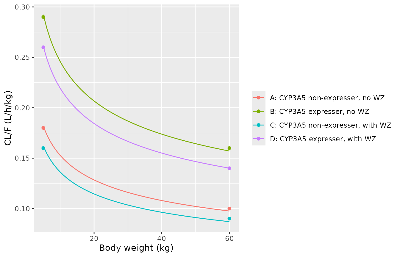
Typical CL/F per kg by body weight and group (lines); points are Figure 2 of Chen 2020 digitised at 5 and 60 kg. Replicates Figure 2 of Chen 2020.
Target attainment (Figure 3 and Table 4)
Chen 2020 simulated each of the four groups at seven body weights (5-60 kg) and nine daily doses (0.01-0.40 mg/kg/day, split into two doses), 1,000 times each, and plotted the probability that the tacrolimus concentration falls in the 5-20 ng/mL target range (Figure 3). The simulation time is not stated; the steady-state pre-dose trough is used here (see Assumptions).
The model is linear in dose, so each weight-by-group arm is simulated
once at 1 mg/kg/day and the trough rescaled for each dose. Each arm has
200 virtual subjects whose V/F random effects are placed at the 200
evenly spaced quantiles of their normal distribution rather than drawn
at random, which makes the target-attainment percentages deterministic.
Residual error is not added (the model’s Cc is the
individual prediction); the Assumptions section explains why.
nsub <- 200
tau <- 12
ndose <- 28 # 14 days twice daily; > 10 V/F-tail half-lives at 60 kg
t_obs <- ndose * tau
om_v <- sqrt(rxode2::rxode(mod)$omega["etalvc", "etalvc"])
#> ℹ parameter labels from comments will be replaced by 'label()'

arms <- tidyr::expand_grid(groups, WT = weights) |>
  mutate(arm = row_number())
subj <- tidyr::expand_grid(arm = arms$arm, k = seq_len(nsub)) |>
  mutate(id = row_number(), etalvc = om_v * qnorm(ppoints(nsub))[k]) |>
  left_join(arms, by = "arm")

ev_pta <- bind_rows(
  tidyr::expand_grid(id = subj$id, time = seq(0, by = tau, length.out = ndose)) |>
    mutate(evid = 1L, cmt = "depot"),
  tibble(id = subj$id, time = t_obs, evid = 0L, cmt = "central")
) |>
  left_join(select(subj, id, WT, CYP3A5_EXPR, CONMED_WUZHI, group), by = "id") |>
  mutate(amt = ifelse(evid == 1L, 1 * WT / 2, 0)) |> # 1 mg/kg/day split in two
  arrange(id, time, desc(evid))

# The etas are supplied per subject, so rxode2 draws none itself.
sim_pta <- suppressWarnings(rxode2::rxSolve(
  mod,
  events = ev_pta, params = select(subj, id, etalvc),
  keep = c("group", "WT")
)) |>
  as.data.frame()
#> ℹ parameter labels from comments will be replaced by 'label()'

dose_levels <- c(0.01, 0.05, 0.10, 0.15, 0.20, 0.25, 0.30, 0.35, 0.40)
pta <- tidyr::expand_grid(sim_pta |> select(id, group, WT, Cc), dose = dose_levels) |>
  mutate(trough = Cc * dose) |>
  group_by(group, WT, dose) |>
  summarise(pta = 100 * mean(trough >= 5 & trough <= 20), .groups = "drop")
# Figure 3 of Chen 2020, digitised by the maintainers (weights 5, 10, 20, ..., 60 kg)
fig3 <- tibble::tribble(
  ~group, ~dose, ~p5, ~p10, ~p20, ~p30, ~p40, ~p50, ~p60,
  "A", 0.05, 33, 67, 90, 94, 97, 98, 98,
  "A", 0.10, 82, 93, 79, 53, 36, 24, 17,
  "A", 0.15, 85, 60, 25, 13, 7, 5, 3,
  "B", 0.05, 0, 1, 13, 27, 42, 54, 62,
  "B", 0.10, 14, 36, 65, 79, 85, 90, 92,
  "B", 0.15, 34, 65, 82, 86, 80, 74, 67,
  "C", 0.05, 56, 83, 95, 98, 98, 99, 100,
  "C", 0.10, 92, 90, 50, 26, 16, 9, 7,
  "C", 0.15, 72, 36, 11, 6, 3, 2, 2,
  "D", 0.05, 0, 7, 30, 51, 64, 74, 80,
  "D", 0.10, 27, 58, 81, 90, 93, 95, 93,
  "D", 0.15, 53, 80, 86, 76, 64, 51, 43
) |>
  tidyr::pivot_longer(starts_with("p"), names_to = "WT", values_to = "fig3_pta") |>
  mutate(WT = as.numeric(sub("p", "", WT)))

pta |>
  left_join(groups, by = "group") |>
  ggplot(aes(WT, pta, colour = factor(dose))) +
  geom_line() +
  geom_point(data = left_join(fig3, groups, by = "group"), aes(y = fig3_pta)) +
  facet_wrap(~label) +
  labs(
    x = "Body weight (kg)", y = "P(5 <= trough <= 20 ng/mL) (%)",
    colour = "Dose (mg/kg/day)"
  )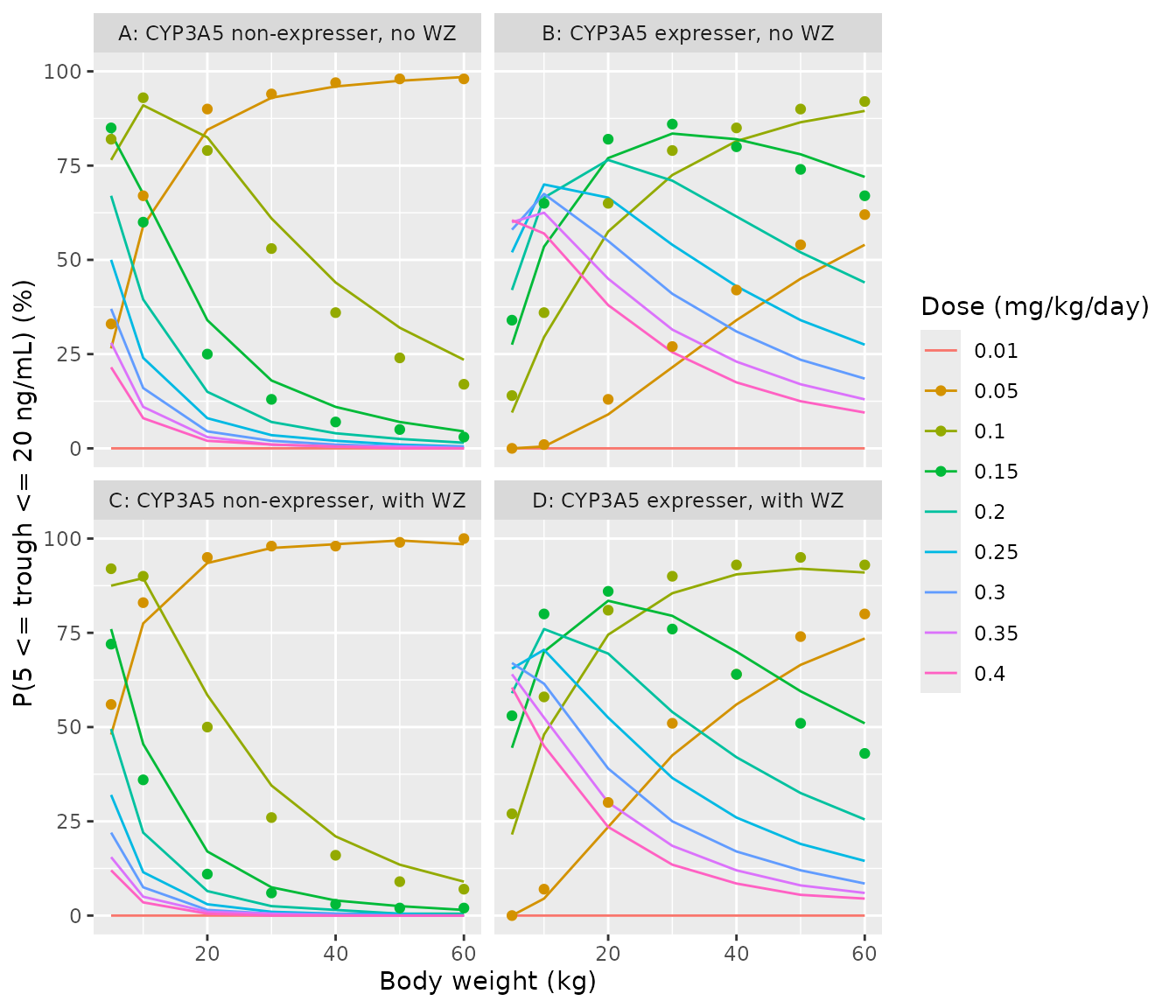
Simulated probability of a steady-state trough in 5-20 ng/mL by body weight, daily dose and group (lines); points are Figure 3 of Chen 2020 digitised for 0.05, 0.10 and 0.15 mg/kg/day. Replicates Figure 3 of Chen 2020.
cmp3 <- inner_join(fig3, pta, by = c("group", "dose", "WT")) |>
  mutate(diff = pta - fig3_pta)
cmp3 |>
  group_by(group) |>
  summarise(
    median_abs_diff = median(abs(diff)), max_abs_diff = max(abs(diff)),
    .groups = "drop"
  ) |>
  dplyr::rename(
    "Group" = group, "Median |difference| (percentage points)" = median_abs_diff,
    "Max |difference| (percentage points)" = max_abs_diff
  ) |>
knitr::kable(digits = 1)| Group | Median |difference| (percentage points) | Max |difference| (percentage points) |
|---|---|---|
| A | 5.0 | 9.0 |
| B | 5.0 | 11.5 |
| C | 2.0 | 9.5 |
| D | 6.5 | 10.0 |
# The replication is deterministic (quantile-placed etas, no residual error),
# so these bounds do not depend on the random-number stream. The published
# curves carry their own Monte Carlo noise (1,000 subjects per cell) and a
# digitisation error of about 2 points.
stopifnot(
  median(abs(cmp3$diff)) < 6.5,
  quantile(abs(cmp3$diff), 0.9) < 12
)
The same replication under the alternative readings of Table 3 – omega V/F = 0.396 as a variance rather than an SD, and residual error included in the simulated troughs – matches Figure 3 less well:
# Variance reading: re-solve with etas on sqrt(0.396) instead of 0.396.
sim_var <- suppressWarnings(rxode2::rxSolve(
  mod,
  events = ev_pta,
  params = select(subj, id, etalvc) |> mutate(etalvc = etalvc / om_v * sqrt(0.396)),
  keep = c("group", "WT")
)) |>
  as.data.frame()

sig_prop <- 0.288
sig_add <- 0.720
pta_of <- function(sim, with_ruv) {
  tidyr::expand_grid(sim |> select(id, group, WT, Cc), dose = c(0.05, 0.10, 0.15)) |>
    mutate(
      trough = Cc * dose,
      sd_ruv = sqrt((trough * sig_prop)^2 + sig_add^2),
      p_in = if (with_ruv) {
        pnorm(20, trough, sd_ruv) - pnorm(5, trough, sd_ruv)
      } else {
        as.numeric(trough >= 5 & trough <= 20)
      }
    ) |>
    group_by(group, WT, dose) |>
    summarise(pta = 100 * mean(p_in), .groups = "drop")
}
rmse_of <- function(p) {
  inner_join(fig3, p, by = c("group", "dose", "WT")) |>
    summarise(rmse = sqrt(mean((pta - fig3_pta)^2))) |>
    pull(rmse)
}
scale_cmp <- tibble(
  reading = c(
    "omega as SD, no residual error (used)",
    "omega as SD, with residual error",
    "omega as variance, no residual error",
    "omega as variance, with residual error"
  ),
  rmse = c(
    rmse_of(pta_of(sim_pta, FALSE)), rmse_of(pta_of(sim_pta, TRUE)),
    rmse_of(pta_of(sim_var, FALSE)), rmse_of(pta_of(sim_var, TRUE))
  )
)
scale_cmp |>
  dplyr::rename("Reading of Table 3" = reading, "RMSE vs Figure 3 (percentage points)" = rmse) |>
knitr::kable(digits = 1)| Reading of Table 3 | RMSE vs Figure 3 (percentage points) |
|---|---|
| omega as SD, no residual error (used) | 5.6 |
| omega as SD, with residual error | 10.9 |
| omega as variance, no residual error | 12.3 |
| omega as variance, with residual error | 17.2 |
# The reading used must beat each alternative by a clear margin.
stopifnot(all(scale_cmp$rmse[1] * 1.5 < scale_cmp$rmse[-1]))
Table 4 turns Figure 3 into weight-banded dose recommendations. Taking, at the midpoint of each band, the dose with the highest target attainment:
doses_all <- tibble(dose = dose_levels)
tab4 <- tibble::tribble(
  ~group, ~lo, ~hi, ~recommended,
  "A", 5, 17, 0.10, "A", 17, 60, 0.05,
  "B", 5, 10, 0.25, "B", 10, 17, 0.20, "B", 17, 36, 0.15, "B", 36, 60, 0.10,
  "C", 5, 11, 0.10, "C", 11, 60, 0.05,
  "D", 5, 10, 0.20, "D", 10, 22, 0.15, "D", 22, 60, 0.10
) |>
  mutate(WT = (lo + hi) / 2)

mid <- tab4 |>
  left_join(groups, by = "group") |>
  mutate(id = row_number())
subj_mid <- tidyr::expand_grid(id = mid$id, k = seq_len(nsub)) |>
  mutate(sid = row_number(), etalvc = om_v * qnorm(ppoints(nsub))[k]) |>
  left_join(select(mid, id, WT, CYP3A5_EXPR, CONMED_WUZHI), by = "id")
ev_mid <- bind_rows(
  tidyr::expand_grid(sid = subj_mid$sid, time = seq(0, by = tau, length.out = ndose)) |>
    mutate(evid = 1L, cmt = "depot"),
  tibble(sid = subj_mid$sid, time = t_obs, evid = 0L, cmt = "central")
) |>
  left_join(select(subj_mid, sid, band = id, WT, CYP3A5_EXPR, CONMED_WUZHI), by = "sid") |>
  mutate(amt = ifelse(evid == 1L, WT / 2, 0)) |>
  rename(id = sid) |>
  arrange(id, time, desc(evid))
sim_mid <- suppressWarnings(rxode2::rxSolve(
  mod,
  events = ev_mid, params = select(subj_mid, id = sid, etalvc),
  keep = "band"
)) |>
  as.data.frame()

best <- tidyr::expand_grid(sim_mid |> select(band, Cc), doses_all) |>
  group_by(band, dose) |>
  summarise(pta = 100 * mean(Cc * dose >= 5 & Cc * dose <= 20), .groups = "drop") |>
  group_by(band) |>
  slice_max(pta, n = 1, with_ties = FALSE) |>
  ungroup()

cmp4 <- mid |>
  left_join(best, by = c("id" = "band")) |>
  mutate(match = abs(dose - recommended) < 1e-9)
cmp4 |>
  select(label, lo, hi, WT, recommended, dose, pta) |>
  mutate(band = paste0(lo, "-", hi)) |>
  select(label, band, WT, recommended, dose, pta) |>
  dplyr::rename(
    "Group" = label, "Band (kg)" = band, "Midpoint (kg)" = WT,
    "Table 4 dose (mg/kg/day)" = recommended,
    "Highest-attainment dose (mg/kg/day)" = dose, "Attainment (%)" = pta
  ) |>
knitr::kable(digits = 2, caption = "Table 4 of Chen 2020 against the highest-attainment simulated dose at each band midpoint.")| Group | Band (kg) | Midpoint (kg) | Table 4 dose (mg/kg/day) | Highest-attainment dose (mg/kg/day) | Attainment (%) |
|---|---|---|---|---|---|
| A: CYP3A5 non-expresser, no WZ | 5-17 | 11.0 | 0.10 | 0.10 | 92.0 |
| A: CYP3A5 non-expresser, no WZ | 17-60 | 38.5 | 0.05 | 0.05 | 96.0 |
| B: CYP3A5 expresser, no WZ | 5-10 | 7.5 | 0.25 | 0.30 | 66.5 |
| B: CYP3A5 expresser, no WZ | 10-17 | 13.5 | 0.20 | 0.20 | 74.0 |
| B: CYP3A5 expresser, no WZ | 17-36 | 26.5 | 0.15 | 0.15 | 82.5 |
| B: CYP3A5 expresser, no WZ | 36-60 | 48.0 | 0.10 | 0.10 | 85.5 |
| C: CYP3A5 non-expresser, with WZ | 5-11 | 8.0 | 0.10 | 0.10 | 92.0 |
| C: CYP3A5 non-expresser, with WZ | 11-60 | 35.5 | 0.05 | 0.05 | 98.5 |
| D: CYP3A5 expresser, with WZ | 5-10 | 7.5 | 0.20 | 0.25 | 71.5 |
| D: CYP3A5 expresser, with WZ | 10-22 | 16.0 | 0.15 | 0.15 | 82.0 |
| D: CYP3A5 expresser, with WZ | 22-60 | 41.0 | 0.10 | 0.10 | 90.5 |
PKNCA validation
The paper reports no NCA. As a structural check, typical-value
subjects (zeroRe()) of 13 kg (the cohort median) in each
group receive the Table 4 dose for that weight for 14 days; PKNCA
computes the steady-state AUC over the last dosing interval, which must
equal the closed form Dose / (CL/F).
nca_grp <- groups |>
  mutate(
    id = row_number(), WT = 13,
    daily = c(0.10, 0.20, 0.05, 0.15), # Table 4 dose at 13 kg
    amt = daily * WT / 2,
    treatment = label
  )
t_last <- (ndose - 1) * tau
ev_nca <- bind_rows(
  tidyr::expand_grid(id = nca_grp$id, time = seq(0, by = tau, length.out = ndose)) |>
    mutate(evid = 1L, cmt = "depot"),
  tidyr::expand_grid(
    id = nca_grp$id,
    time = t_last + c(0, 0.1, 0.25, 0.5, 0.75, 1, 1.5, 2, 3, 4, 6, 8, 10, 12)
  ) |>
    mutate(evid = 0L, cmt = "central")
) |>
  left_join(select(nca_grp, id, WT, CYP3A5_EXPR, CONMED_WUZHI, treatment, dose_amt = amt), by = "id") |>
  mutate(amt = ifelse(evid == 1L, dose_amt, 0)) |>
  select(-dose_amt) |>
  arrange(id, time, desc(evid))

sim_nca <- rxode2::rxSolve(mod_typ, events = ev_nca, keep = "treatment") |>
  as.data.frame()
#> ℹ omega/sigma items treated as zero: 'etalvc'
#> Warning: multi-subject simulation without without 'omega'

conc <- sim_nca |>
  filter(!is.na(Cc), time >= t_last) |>
  select(id, time, Cc, treatment)
doses_nca <- ev_nca |>
  filter(evid == 1L, time == t_last) |>
  select(id, time, amt, treatment)

o_conc <- PKNCAconc(conc, Cc ~ time | treatment + id)
o_dose <- PKNCAdose(doses_nca, amt ~ time | treatment + id)
intervals <- data.frame(start = t_last, end = t_last + tau, auclast = TRUE, cmax = TRUE, cmin = TRUE)
nca_res <- pk.nca(PKNCAdata(o_conc, o_dose, intervals = intervals))

cl_13 <- sim_nca |>
  filter(time == t_last) |>
  distinct(treatment, cl)
nca_wide <- as.data.frame(nca_res) |>
  select(treatment, PPTESTCD, PPORRES) |>
  tidyr::pivot_wider(names_from = PPTESTCD, values_from = PPORRES) |>
  left_join(select(nca_grp, treatment, amt), by = "treatment") |>
  left_join(cl_13, by = "treatment") |>
  mutate(auc_closed = 1000 * amt / cl)

nca_wide |>
  select(treatment, amt, cmax, cmin, auclast, auc_closed) |>
  dplyr::rename(
    "Group" = treatment, "Dose (mg q12h)" = amt, "Cmax (ng/mL)" = cmax,
    "Cmin (ng/mL)" = cmin, "AUCtau (PKNCA, ng*h/mL)" = auclast,
    "Dose/(CL/F) (ng*h/mL)" = auc_closed
  ) |>
knitr::kable(digits = 2, caption = "Typical-value steady-state NCA at 13 kg on the Table 4 dose.")| Group | Dose (mg q12h) | Cmax (ng/mL) | Cmin (ng/mL) | AUCtau (PKNCA, ng*h/mL) | Dose/(CL/F) (ng*h/mL) |
|---|---|---|---|---|---|
| A: CYP3A5 non-expresser, no WZ | 0.65 | 51.94 | 12.55 | 349.16 | 349.71 |
| B: CYP3A5 expresser, no WZ | 1.30 | 84.97 | 8.54 | 433.30 | 434.43 |
| C: CYP3A5 non-expresser, with WZ | 0.32 | 27.56 | 7.78 | 195.75 | 196.03 |
| D: CYP3A5 expresser, with WZ | 0.98 | 66.43 | 8.57 | 364.43 | 365.27 |
Assumptions and deviations
-
IIV and residual-error scale. Table 3 reports
“omega V/F = 0.396”, “sigma 1 = 0.288” (proportional) and “sigma 2 =
0.720” (additive) without stating whether they are variances or standard
deviations. Replicating the Figure 3 target-attainment curves settles
it. With 0.396 as the SD of the V/F random effect and no residual error,
the deterministic replication above reproduces the digitised curves with
a root-mean-square error of about 6 percentage points across all four
panels; reading 0.396 as a variance (SD 0.63) roughly doubles that error
(table above), and the wider variance reading cannot produce the
near-certain attainment the paper shows at 0.05 mg/kg/day above 40 kg in
group A (published 97-98%). The SD reading is used, and sigma 1 and
sigma 2 are read on the same scale as omega in the same table
(proportional SD 28.8%, additive SD 0.72 ng/mL). This matches the scale
settled for an earlier model by the same group
(
Wang_2019b_tacrolimus, also by replicating the paper’s own simulations). - Residual error in Figure 3. Adding the residual error to the simulated troughs widens the distribution and roughly doubles the error against Figure 3 (table above), so the published simulations appear to be of individual predictions. The replication above excludes residual error accordingly; the model file keeps it for simulating observations.
- Simulation time for Figure 3. Not stated. The steady-state pre-dose trough (12 h after a dose, day 14 of twice-daily dosing) reproduces the curves; a trough after only the first few doses does not.
- Table 4 in the lightest CYP3A5*1 carriers. At the 7.5 kg midpoint of the 5-10 kg bands in groups B and D the replication’s highest-attainment dose is one 0.05 mg/kg/day step above Table 4 (table above). In Figure 3B and 3D the two or three highest-attainment doses lie within a few percentage points of each other below 10 kg, so the choice between adjacent dose steps there is within the Monte Carlo noise of 1,000 simulated subjects per cell.
- No IIV on CL/F. Table 3 reports a random effect on V/F only; none is estimated on CL/F. This is reproduced as published.
-
Wuzhi-capsule effect form. Eq. 7 prints the effect
as
(1 - 0.108 x WZ), the Methods Eq. 6 form(1 + theta x COV)with theta = -0.108. The Wuzhi-capsule indicator is taken per record; the paper does not say whether it varied within a patient. - Fixed ka. 4.48 1/h is taken from earlier paediatric liver-transplant models (Chen 2020 refs 23 and 25) and was not estimated.
- Reference weight. The 70 kg reference lies far outside the observed 6.4-28 kg range, so 6.57 L/h and 77.6 L are adult-equivalent extrapolations.
- Small cohort. The model was fitted to 12 children; the bootstrap intervals in Table 3 are wide (e.g. V/F 15.6-501.9 L), and the authors call for external validation.