Cefotaxime (Hartman 2022)
Source:vignettes/articles/Hartman_2022_cefotaxime.Rmd
Hartman_2022_cefotaxime.RmdModel and source
- Citation: Hartman SJF, Upadhyay PJ, Mathot RAA, van der Flier M, Schreuder MF, Bruggemann RJ, Knibbe CAJ, de Wildt SN. Population pharmacokinetics of intravenous cefotaxime indicates that higher doses are required for critically ill children. J Antimicrob Chemother. 2022;77(6):1725-1732. doi:10.1093/jac/dkac095. The open-access supplementary data (dkac095_supplementary_data.docx, retrieved from EuropePMC PMC9155601) provides the final NONMEM control stream used to confirm the model structure, the parameter scales and the residual-error form, and Figure S6 used for the dose-evaluation replication in the vignette.
- Description: Two-compartment population PK model with first-order elimination for intravenous cefotaxime in critically ill children (0-18 years) admitted to a paediatric intensive care unit (POPSICLE study, Radboudumc, the Netherlands). Clearance and central volume carry estimated power functions of body weight normalised to the cohort median of 10.95 kg (exponents 1.11 and 1.18); peripheral volume and inter-compartmental clearance are not weight-scaled. Correlated log-normal interindividual variability on clearance and central volume; log-normal (exponential) residual error (Hartman 2022).
- Article: https://doi.org/10.1093/jac/dkac095 (open access, PMC9155601)
- Supplement: Supplementary data (methods, Figures S1-S6 and the final NONMEM control stream), available from the article page at JAC Online and from Europe PMC.
Hartman et al. characterised the pharmacokinetics of intravenous cefotaxime in critically ill children and used the final model to evaluate current and alternative dosing regimens against a 100% fT>MIC target (trough unbound concentration above the MIC) for MICs of 0.5, 2 and 4 mg/L.
Population
The analysis included 52 children (median postnatal age 1.61 years, range 0.03-17.69 years; median weight 10.95 kg, range 2.7-80 kg; 38.5% female) admitted to the level-3 paediatric intensive care unit of the Radboudumc (Nijmegen, the Netherlands) between June 2017 and May 2019 as part of the POPSICLE study (NCT03248349). The main reasons for admission were respiratory failure (63.5%), neurological impairment (17.3%) and circulatory failure (9.6%); 90.4% were mechanically ventilated and 36.5% received vasopressive co-medication during the study. Most children received the prophylactic dose of 100 mg/kg/day (maximum 4 g/day, selective decontamination of the digestive tract); 11 (21.2%) received the therapeutic dose of 150 mg/kg/day (maximum 12 g/day), as three or four intravenous push doses per day. In total 479 total plasma cefotaxime concentrations (median 10 per patient) entered the final model. Demographics are from Table 1 of Hartman 2022; the cohort was predominantly Caucasian (>90%).
The same information is available programmatically:
str(rxode2::rxode(readModelDb("Hartman_2022_cefotaxime"))$population)
#> List of 13
#>  $ species       : chr "human"
#>  $ n_subjects    : num 52
#>  $ n_studies     : num 1
#>  $ n_observations: num 479
#>  $ age_range     : chr "0.03-17.69 years (median 1.61, IQR 0.17-8.63)"
#>  $ weight_range  : chr "2.7-80 kg (median 10.95, IQR 5.2-28.5)"
#>  $ sex_female_pct: num 38.5
#>  $ race_ethnicity: chr "Predominantly Caucasian (>90%; Discussion 'Limitations')."
#>  $ disease_state : chr "Critically ill children in a level-3 paediatric intensive care unit receiving intravenous cefotaxime; main admi"| __truncated__
#>  $ dose_range    : chr "Prophylactic 100 mg/kg/day (maximum 4 g/day; selective decontamination of the digestive tract) or therapeutic 1"| __truncated__
#>  $ renal_function: chr "Baseline serum creatinine median 28 (range 8-87) umol/L; baseline Schwartz-2012 eGFR median 89 (range 46-398) mL/min/1.73 m2."
#>  $ regions       : chr "Netherlands (Radboudumc, Nijmegen; single centre)."
#>  $ notes         : chr "POPSICLE study (NCT03248349), June 2017 - May 2019. Rich sampling (median 10 samples per patient) over up to 14"| __truncated__
Source trace
Every ini() value carries an in-file comment pointing to
its source. The final NONMEM control stream in the supplement confirms
the structure (ADVAN5, two compartments, weight on CL and V1 only,
Y = F*EXP(EPS(1))).
| Equation / parameter | Value | Source location |
|---|---|---|
lcl (CL at 10.95 kg) |
log(2.8) L/h | Table 2, CLpop |
lvc (V1 at 10.95 kg) |
log(2.62) L | Table 2, V1pop |
lvp (V2) |
log(1.55) L | Table 2, V2pop |
lq (Q) |
log(1.15) L/h | Table 2, Qpop |
e_wt_cl |
1.11 | Table 2, Theta1 |
e_wt_vc |
1.18 | Table 2, Theta2 |
etalcl variance |
0.359 | Table 2, IIV CL; 65.7% CV in Results |
etalcl-etalvc covariance |
0.305 | Table 2, ‘Block matrix’ |
etalvc variance |
0.581 | Table 2, IIV V1; 88.8% CV in Results |
expSd |
sqrt(0.307) | Table 2, ‘Proportional error’ (raw $SIGMA variance) |
CL = CLpop * (WT/10.95)^Theta1 * exp(eta) |
n/a | Table 2 equation; control stream $PK |
V1 = V1pop * (WT/10.95)^Theta2 * exp(eta) |
n/a | Table 2 equation; control stream $PK |
V2 = V2pop, Q = Qpop (no weight
scaling) |
n/a | Control stream $PK (V2 = TVV2,
Q = TVQ) |
d/dt(central), d/dt(peripheral1)
|
n/a | Control stream $DES (ADVAN5 K10, K12, K21) |
Cc ~ lnorm(expSd) |
n/a | Control stream $ERROR Y = F*EXP(EPS(1)); supplementary
results |
Checks against the published numbers
The Discussion quotes the typical clearance and total volume per
kilogram at the cohort median weight (0.26 L/kg/h and 0.38 L/kg), and
the Results quote the final-model IIV as 65.7% (CL) and 88.8% (V1).
These are deterministic functions of the ini() values and
are checked exactly.
ui <- rxode2::rxode(readModelDb("Hartman_2022_cefotaxime"))
th <- ui$theta
om <- ui$omega

cl_per_kg <- exp(th[["lcl"]]) / 10.95
vd_per_kg <- (exp(th[["lvc"]]) + exp(th[["lvp"]])) / 10.95
cv_cl <- 100 * sqrt(exp(om["etalcl", "etalcl"]) - 1)
cv_vc <- 100 * sqrt(exp(om["etalvc", "etalvc"]) - 1)
corr_cl_vc <- om["etalcl", "etalvc"] / sqrt(om["etalcl", "etalcl"] * om["etalvc", "etalvc"])

knitr::kable(
  data.frame(
    Quantity = c("CL per kg (L/kg/h)", "Vd per kg (L/kg)", "IIV CL (%CV)", "IIV V1 (%CV)", "CL-V1 correlation"),
    Model = signif(c(cl_per_kg, vd_per_kg, cv_cl, cv_vc, corr_cl_vc), 3),
    Paper = c("0.26", "0.38", "65.7", "88.8", "not reported")
  ),
  caption = "Typical values and IIV implied by the model against the values quoted in Hartman 2022."
)| Quantity | Model | Paper |
|---|---|---|
| CL per kg (L/kg/h) | 0.256 | 0.26 |
| Vd per kg (L/kg) | 0.381 | 0.38 |
| IIV CL (%CV) | 65.700 | 65.7 |
| IIV V1 (%CV) | 88.800 | 88.8 |
| CL-V1 correlation | 0.668 | not reported |
Dose evaluation in typical patients (Figure 2 and Figure S6)
The paper’s dose evaluations use five typical patients with a normal weight for age (1 week 3.775 kg, 1 year 9.75 kg, 4 years 17.125 kg, 8 years 26.75 kg, 18 years 60.5 kg), a maximum daily dose of 12 g, unbound concentrations taken as 60% of total, and the trough 24 h after the first dose as the surrogate for fT>MIC. The continuous-infusion regimens start with a 25 mg/kg loading dose (maximum 1000 mg).
typical <- tibble::tibble(
  patient = c("1 week - 3.775 kg", "1 year - 9.75 kg", "4 year - 17.125 kg", "8 year - 26.75 kg", "18 years - 60.5 kg"),
  WT = c(3.775, 9.75, 17.125, 26.75, 60.5)
)

regimens <- tibble::tribble(
  ~regimen, ~mgkgday, ~tau, ~dur,
  "150 mg/kg/day bolus q8h", 150, 8, 0,
  "200 mg/kg/day bolus q6h", 200, 6, 0,
  "150 mg/kg/day bolus q4h", 150, 4, 0,
  "200 mg/kg/day bolus q4h", 200, 4, 0,
  "150 mg/kg/day 60-min infusion q8h", 150, 8, 1,
  "200 mg/kg/day 60-min infusion q6h", 200, 6, 1,
  "150 mg/kg/day 120-min infusion q8h", 150, 8, 2,
  "200 mg/kg/day 120-min infusion q6h", 200, 6, 2,
  "150 mg/kg/day 240-min infusion q8h", 150, 8, 4,
  "200 mg/kg/day 240-min infusion q6h", 200, 6, 4,
  "100 mg/kg/day continuous + 25 mg/kg LD", 100, 24, 24,
  "150 mg/kg/day continuous + 25 mg/kg LD", 150, 24, 24,
  "200 mg/kg/day continuous + 25 mg/kg LD", 200, 24, 24
)

obs_times <- sort(unique(c(seq(0, 24, by = 0.1), 24)))

make_typical_events <- function(regimen_row, typical, obs_times) {
  rows <- vector("list", nrow(typical))
  for (i in seq_len(nrow(typical))) {
    wt <- typical$WT[i]
    daily <- min(regimen_row$mgkgday * wt, 12000)
    dose_times <- seq(0, 24 - regimen_row$tau, by = regimen_row$tau)
    amt <- daily / length(dose_times)
    doses <- tibble::tibble(time = dose_times, amt = amt, evid = 1L, rate = 0)
    if (regimen_row$dur > 0) {
      doses$rate <- amt / regimen_row$dur
    }
    if (regimen_row$dur == 24) {
      # Continuous infusion: 25 mg/kg (maximum 1000 mg) loading bolus plus the
      # daily dose infused over 24 h.
      doses <- dplyr::bind_rows(
        tibble::tibble(time = 0, amt = min(25 * wt, 1000), evid = 1L, rate = 0),
        doses
      )
    }
    obs <- tibble::tibble(time = obs_times, amt = NA_real_, evid = 0L, rate = NA_real_)
    rows[[i]] <- dplyr::bind_rows(doses, obs) |>
      dplyr::mutate(patient = typical$patient[i], WT = wt, cmt = "central")
  }
  dplyr::bind_rows(rows) |> dplyr::mutate(regimen = regimen_row$regimen)
}

typical_events <- dplyr::bind_rows(lapply(seq_len(nrow(regimens)), function(j) {
  make_typical_events(regimens[j, ], typical, obs_times)
})) |>
  dplyr::mutate(id = as.integer(factor(paste(regimen, patient), levels = unique(paste(regimen, patient))))) |>
  dplyr::arrange(id, time, dplyr::desc(evid))

stopifnot(length(unique(typical_events$id)) == nrow(regimens) * nrow(typical))
mod <- readModelDb("Hartman_2022_cefotaxime")
mod_typical <- rxode2::zeroRe(mod)
# zeroRe() leaves a multi-subject solve with no omega; rxode2 warns about
# exactly that, which is the intent here.
sim_typical <- suppressWarnings(rxode2::rxSolve(
  mod_typical,
  events = typical_events,
  keep = c("regimen", "patient")
)) |>
  as.data.frame() |>
  dplyr::mutate(Cu = 0.6 * Cc)
#> ℹ omega/sigma items treated as zero: 'etalcl', 'etalvc'

# Pre-dose rows are exactly zero and cannot be drawn on a log axis.
sim_plot <- sim_typical |>
  dplyr::mutate(Cu = dplyr::if_else(Cu > 0, Cu, NA_real_))
mic_lines <- data.frame(MIC = c(0.5, 2, 4), label = c("MIC 0.5 mg/L", "MIC 2 mg/L", "MIC 4 mg/L"))
fig2_regimens <- c(
  "200 mg/kg/day bolus q6h",
  "200 mg/kg/day bolus q4h",
  "200 mg/kg/day continuous + 25 mg/kg LD"
)
sim_plot |>
  dplyr::filter(regimen %in% fig2_regimens) |>
  dplyr::mutate(
    regimen = factor(regimen, levels = fig2_regimens),
    patient = factor(patient, levels = typical$patient)
  ) |>
  ggplot(aes(time, Cu, colour = patient)) +
  geom_line(na.rm = TRUE) +
  geom_hline(data = mic_lines, aes(yintercept = MIC, linetype = label)) +
  facet_wrap(~regimen) +
  scale_y_log10(limits = c(0.01, 1000)) +
  labs(
    x = "Time (h)", y = "Unbound cefotaxime (mg/L)", colour = "Typical patient", linetype = NULL,
    title = "Typical-patient unbound concentrations, three regimens",
    caption = "Replicates Figure 2 of Hartman 2022 (unbound = 0.6 x total)."
  ) +
  theme(legend.position = "bottom")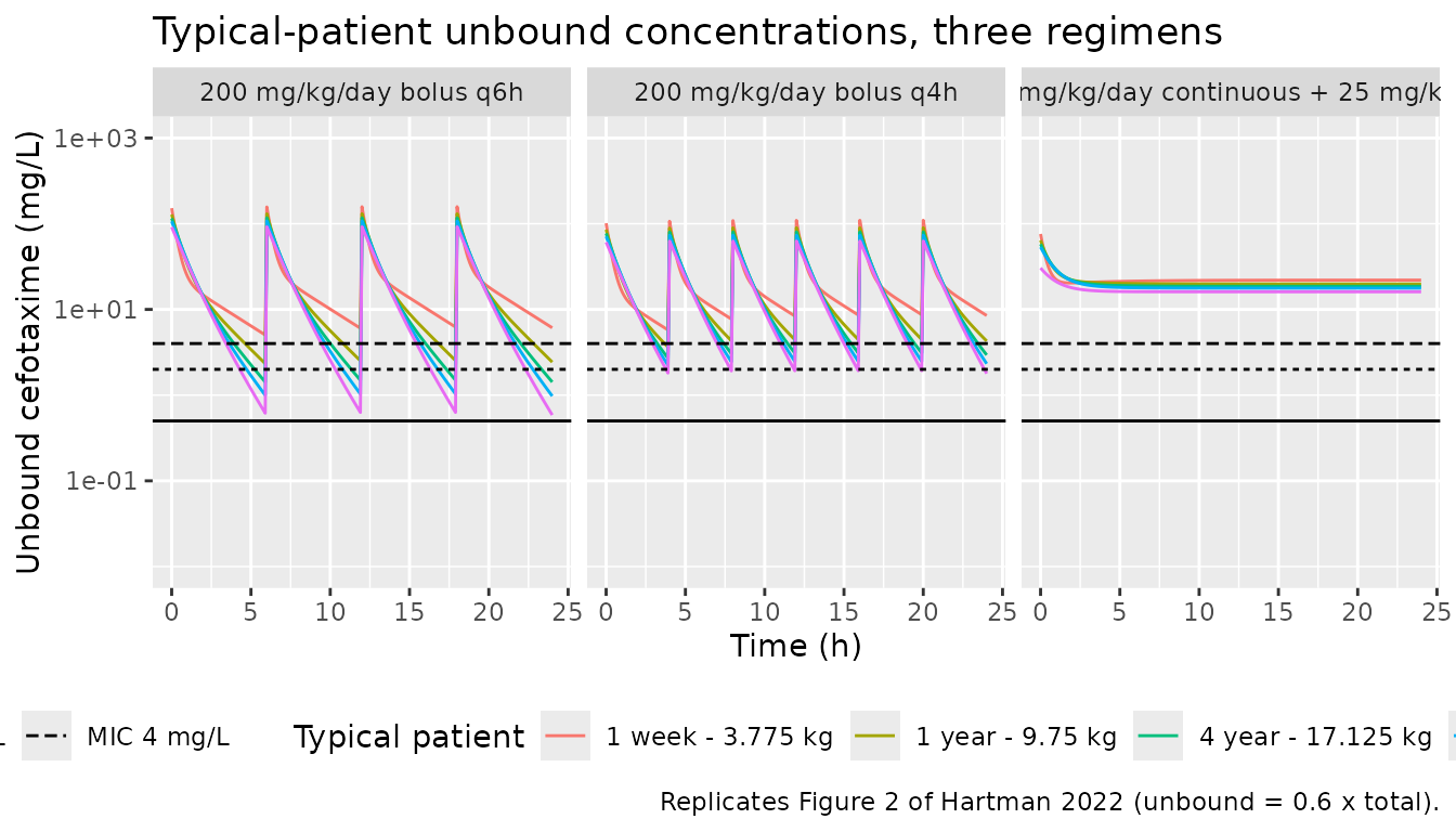
sim_plot |>
  dplyr::mutate(
    regimen = factor(regimen, levels = regimens$regimen),
    patient = factor(patient, levels = typical$patient)
  ) |>
  ggplot(aes(time, Cu, colour = patient)) +
  geom_line(na.rm = TRUE) +
  geom_hline(data = mic_lines, aes(yintercept = MIC, linetype = label)) +
  facet_wrap(~regimen, ncol = 2) +
  scale_y_log10(limits = c(0.01, 1000)) +
  labs(
    x = "Time (h)", y = "Unbound cefotaxime (mg/L)", colour = "Typical patient", linetype = NULL,
    title = "All evaluated regimens",
    caption = "Replicates Figure S6 of Hartman 2022 (unbound = 0.6 x total)."
  ) +
  theme(legend.position = "bottom")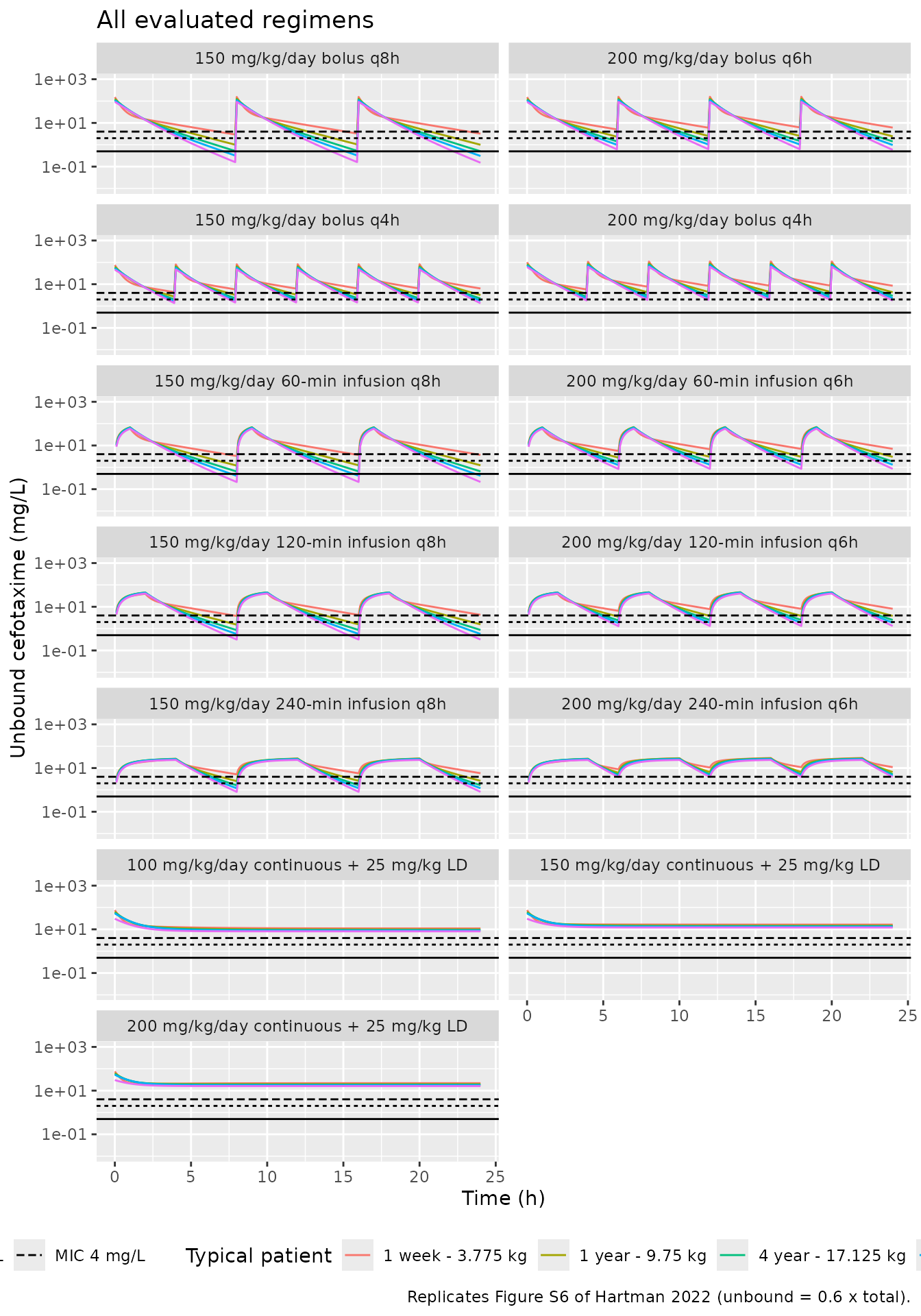
Trough concentrations at 24 h
The paper reports its conclusions graphically. The reference values below were digitised by the maintainers from the 24 h trough points of the bolus panels of Figure S6 (log axis; reading precision roughly +/-10%) and from the plateaus of the continuous-infusion panels.
troughs <- sim_typical |>
  dplyr::filter(time == 24) |>
  dplyr::select(regimen, patient, Cu)

digitised <- tibble::tribble(
  ~regimen, ~patient, ~Cu_fig,
  "150 mg/kg/day bolus q8h", "1 week - 3.775 kg", 3.0,
  "150 mg/kg/day bolus q8h", "1 year - 9.75 kg", 1.0,
  "150 mg/kg/day bolus q8h", "4 year - 17.125 kg", 0.5,
  "150 mg/kg/day bolus q8h", "8 year - 26.75 kg", 0.3,
  "150 mg/kg/day bolus q8h", "18 years - 60.5 kg", 0.15,
  "200 mg/kg/day bolus q6h", "1 week - 3.775 kg", 6.0,
  "200 mg/kg/day bolus q6h", "1 year - 9.75 kg", 2.5,
  "200 mg/kg/day bolus q6h", "4 year - 17.125 kg", 1.4,
  "200 mg/kg/day bolus q6h", "8 year - 26.75 kg", 1.0,
  "200 mg/kg/day bolus q6h", "18 years - 60.5 kg", 0.6,
  "150 mg/kg/day bolus q4h", "1 week - 3.775 kg", 6.0,
  "150 mg/kg/day bolus q4h", "1 year - 9.75 kg", 3.0,
  "150 mg/kg/day bolus q4h", "4 year - 17.125 kg", 2.0,
  "150 mg/kg/day bolus q4h", "8 year - 26.75 kg", 1.6,
  "150 mg/kg/day bolus q4h", "18 years - 60.5 kg", 1.35,
  "200 mg/kg/day bolus q4h", "1 week - 3.775 kg", 8.5,
  "200 mg/kg/day bolus q4h", "1 year - 9.75 kg", 3.8,
  "200 mg/kg/day bolus q4h", "4 year - 17.125 kg", 2.5,
  "200 mg/kg/day bolus q4h", "8 year - 26.75 kg", 2.1,
  "200 mg/kg/day bolus q4h", "18 years - 60.5 kg", 1.8,
  "200 mg/kg/day continuous + 25 mg/kg LD", "1 week - 3.775 kg", 22,
  "200 mg/kg/day continuous + 25 mg/kg LD", "18 years - 60.5 kg", 17
)

trough_cmp <- digitised |>
  dplyr::left_join(troughs, by = c("regimen", "patient")) |>
  dplyr::mutate(pct_diff = 100 * (Cu / Cu_fig - 1))
stopifnot(nrow(trough_cmp) == nrow(digitised), !anyNA(trough_cmp$Cu))

trough_cmp |>
  dplyr::mutate(Cu = signif(Cu, 3), pct_diff = round(pct_diff, 1)) |>
  dplyr::rename(
    "Regimen" = regimen,
    "Typical patient" = patient,
    "Figure S6 (mg/L)" = Cu_fig,
    "Model (mg/L)" = Cu,
    "Difference (%)" = pct_diff
  ) |>
knitr::kable(caption = "Unbound trough at 24 h: model versus values digitised from Figure S6.")| Regimen | Typical patient | Figure S6 (mg/L) | Model (mg/L) | Difference (%) |
|---|---|---|---|---|
| 150 mg/kg/day bolus q8h | 1 week - 3.775 kg | 3.00 | 3.230 | 7.6 |
| 150 mg/kg/day bolus q8h | 1 year - 9.75 kg | 1.00 | 0.999 | -0.1 |
| 150 mg/kg/day bolus q8h | 4 year - 17.125 kg | 0.50 | 0.503 | 0.7 |
| 150 mg/kg/day bolus q8h | 8 year - 26.75 kg | 0.30 | 0.308 | 2.6 |
| 150 mg/kg/day bolus q8h | 18 years - 60.5 kg | 0.15 | 0.151 | 0.6 |
| 200 mg/kg/day bolus q6h | 1 week - 3.775 kg | 6.00 | 6.110 | 1.8 |
| 200 mg/kg/day bolus q6h | 1 year - 9.75 kg | 2.50 | 2.430 | -2.8 |
| 200 mg/kg/day bolus q6h | 4 year - 17.125 kg | 1.40 | 1.420 | 1.6 |
| 200 mg/kg/day bolus q6h | 8 year - 26.75 kg | 1.00 | 0.975 | -2.5 |
| 200 mg/kg/day bolus q6h | 18 years - 60.5 kg | 0.60 | 0.587 | -2.2 |
| 150 mg/kg/day bolus q4h | 1 week - 3.775 kg | 6.00 | 6.360 | 6.0 |
| 150 mg/kg/day bolus q4h | 1 year - 9.75 kg | 3.00 | 3.210 | 6.8 |
| 150 mg/kg/day bolus q4h | 4 year - 17.125 kg | 2.00 | 2.210 | 10.3 |
| 150 mg/kg/day bolus q4h | 8 year - 26.75 kg | 1.60 | 1.740 | 9.0 |
| 150 mg/kg/day bolus q4h | 18 years - 60.5 kg | 1.35 | 1.350 | -0.1 |
| 200 mg/kg/day bolus q4h | 1 week - 3.775 kg | 8.50 | 8.480 | -0.2 |
| 200 mg/kg/day bolus q4h | 1 year - 9.75 kg | 3.80 | 4.270 | 12.5 |
| 200 mg/kg/day bolus q4h | 4 year - 17.125 kg | 2.50 | 2.940 | 17.7 |
| 200 mg/kg/day bolus q4h | 8 year - 26.75 kg | 2.10 | 2.320 | 10.7 |
| 200 mg/kg/day bolus q4h | 18 years - 60.5 kg | 1.80 | 1.780 | -0.9 |
| 200 mg/kg/day continuous + 25 mg/kg LD | 1 week - 3.775 kg | 22.00 | 22.000 | -0.1 |
| 200 mg/kg/day continuous + 25 mg/kg LD | 18 years - 60.5 kg | 17.00 | 16.100 | -5.5 |
All typical-patient troughs fall within the digitising precision of the figure. The comparison is deterministic (typical values, no random effects), so the bound below does not depend on the simulation seed; a transcription error in a clearance, volume or exponent moves these troughs by far more than 25%.
Dosing conclusions (Results and Table 3)
cu24 <- function(reg, pat_age) {
  v <- troughs$Cu[troughs$regimen == reg & startsWith(troughs$patient, pat_age)]
  if (length(v) != 1L) stop("no unique trough for '", reg, "' / '", pat_age, "'")
  v
}
ages <- c("1 week", "1 year", "4 year", "8 year", "18 years")
q8_150 <- vapply(ages, cu24, numeric(1), reg = "150 mg/kg/day bolus q8h")
q6_200 <- vapply(ages, cu24, numeric(1), reg = "200 mg/kg/day bolus q6h")
q4_200 <- vapply(ages, cu24, numeric(1), reg = "200 mg/kg/day bolus q4h")
ci_200 <- vapply(ages, cu24, numeric(1), reg = "200 mg/kg/day continuous + 25 mg/kg LD")

claims <- tibble::tribble(
  ~claim, ~holds, ~deviation,
  "150 mg/kg/day: trough < 0.5 mg/L in patients > 4 years (8 and 18 years)", all(q8_150[c("8 year", "18 years")] < 0.5), FALSE,
  "200 mg/kg/day q6h: trough > 0.5 mg/L in all typical patients", all(q6_200 > 0.5), FALSE,
  "200 mg/kg/day q6h: trough > 2 mg/L in patients < 1 year (1 week)", q6_200[["1 week"]] > 2, FALSE,
  "200 mg/kg/day q4h: trough > 2 mg/L in all typical patients", all(q4_200 > 2), TRUE,
  "200 mg/kg/day q4h: trough > 2 mg/L in patients 1 week to 8 years", all(q4_200[c("1 week", "1 year", "4 year", "8 year")] > 2), FALSE,
  "200 mg/kg/day q4h: trough > 4 mg/L in patients < 1 year (1 week)", q4_200[["1 week"]] > 4, FALSE,
  "200 mg/kg/day q4h: trough < 4 mg/L in patients > 1 year (CI needed for MIC 4)", all(q4_200[c("4 year", "8 year", "18 years")] < 4), FALSE,
  "25 mg/kg LD + 200 mg/kg/day continuous: > 4 mg/L in all typical patients", all(ci_200 > 4), FALSE
)
claims |>
  dplyr::rename("Claim" = claim, "Reproduced" = holds, "Known deviation" = deviation) |>
knitr::kable(caption = "Dosing conclusions of Hartman 2022 evaluated on the typical-patient simulations.")| Claim | Reproduced | Known deviation |
|---|---|---|
| 150 mg/kg/day: trough < 0.5 mg/L in patients > 4 years (8 and 18 years) | TRUE | FALSE |
| 200 mg/kg/day q6h: trough > 0.5 mg/L in all typical patients | TRUE | FALSE |
| 200 mg/kg/day q6h: trough > 2 mg/L in patients < 1 year (1 week) | TRUE | FALSE |
| 200 mg/kg/day q4h: trough > 2 mg/L in all typical patients | FALSE | TRUE |
| 200 mg/kg/day q4h: trough > 2 mg/L in patients 1 week to 8 years | TRUE | FALSE |
| 200 mg/kg/day q4h: trough > 4 mg/L in patients < 1 year (1 week) | TRUE | FALSE |
| 200 mg/kg/day q4h: trough < 4 mg/L in patients > 1 year (CI needed for MIC 4) | TRUE | FALSE |
| 25 mg/kg LD + 200 mg/kg/day continuous: > 4 mg/L in all typical patients | TRUE | FALSE |
stopifnot(all(claims$holds[!claims$deviation]))
# The one known deviation sits at the MIC line, not far from it: the 18-year-old
# trough on 200 mg/kg/day q4h is just under 2 mg/L, as it is in Figure S6.
stopifnot(q4_200[["18 years"]] > 1.6, q4_200[["18 years"]] < 2)
One conclusion is not reproduced exactly. The Results state that 200 mg/kg/day every 4 h gives adequate troughs for MICs up to 2 mg/L in all typical patients, but the 18-year-old (60.5 kg) trough is 1.78 mg/L unbound. Figure S6 of the paper shows the same thing: the 18-year-old points of the 200 mg/kg/day q4h panel sit just under the 2 mg/L reference line (digitised at about 1.8 mg/L, table above). The statement in the text rounds a near-miss up; the model agrees with the published figure.
Stochastic simulation of the study population
A virtual cohort of 200 children per arm is drawn with a log-normal weight distribution matched to the Table 1 median (10.95 kg) and interquartile range (5.2-28.5 kg), truncated to the observed 2.7-80 kg range. Two arms mirror the study doses: the prophylactic 100 mg/kg/day (maximum 4 g/day) and the therapeutic 150 mg/kg/day (maximum 12 g/day), both as intravenous push doses every 6 h for 3 days.
rxode2::rxSetSeed(2022)
set.seed(2022)
n_per_arm <- 200

draw_wt <- function(n) {
  mu <- log(10.95)
  sdlog <- (log(28.5) - log(5.2)) / (2 * qnorm(0.75))
  out <- numeric(0)
  while (length(out) < n) {
    w <- stats::rlnorm(n, mu, sdlog)
    out <- c(out, w[w >= 2.7 & w <= 80])
  }
  out[seq_len(n)]
}

make_cohort <- function(n, mgkgday, maxday, label, id_offset) {
  subj <- tibble::tibble(id = id_offset + seq_len(n), WT = draw_wt(n), treatment = label)
  dose_times <- seq(0, 66, by = 6)
  obs_times <- sort(unique(c(seq(0, 72, by = 0.5), seq(66, 72, by = 0.05))))
  doses <- tidyr::crossing(subj, time = dose_times) |>
    dplyr::mutate(amt = pmin(mgkgday * WT, maxday) / 4, evid = 1L)
  obs <- tidyr::crossing(subj, time = obs_times) |>
    dplyr::mutate(amt = NA_real_, evid = 0L)
  dplyr::bind_rows(doses, obs) |>
    dplyr::mutate(cmt = "central") |>
    dplyr::arrange(id, time, dplyr::desc(evid))
}

events <- dplyr::bind_rows(
  make_cohort(n_per_arm, 100, 4000, "100 mg/kg/day q6h", 0L),
  make_cohort(n_per_arm, 150, 12000, "150 mg/kg/day q6h", n_per_arm)
)
stopifnot(length(unique(events$id)) == 2 * n_per_arm)
sim <- rxode2::rxSolve(mod, events = events, keep = c("treatment", "WT")) |>
  as.data.frame()
sim |>
  dplyr::filter(time <= 24) |>
  dplyr::group_by(treatment, time) |>
  dplyr::summarise(
    Q05 = quantile(Cc, 0.05), Q50 = median(Cc), Q95 = quantile(Cc, 0.95),
    .groups = "drop"
  ) |>
  ggplot(aes(time, Q50)) +
  geom_ribbon(aes(ymin = Q05, ymax = Q95), alpha = 0.25) +
  geom_line() +
  facet_wrap(~treatment) +
  scale_y_log10() +
  labs(
    x = "Time after first dose (h)", y = "Total cefotaxime (mg/L)",
    title = "Simulated total plasma cefotaxime, first 24 h",
    caption = "Median and 90% prediction interval of the individual predictions."
  )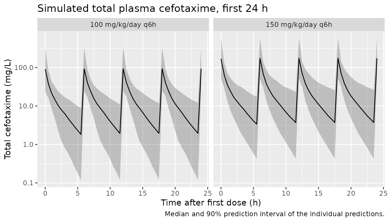
The paper reports an over 10-fold range of observed trough concentrations and individual clearances between 0.02 and 0.66 L/kg/h (Figure S2). The simulated cohort reproduces that breadth; the check is on robust quantiles, not the extremes, so it holds for any draw.
trough_sim <- sim |> dplyr::filter(time == 24)
cl_kg <- sim |>
  dplyr::distinct(id, .keep_all = TRUE) |>
  dplyr::mutate(cl_kg = cl / WT)
spread <- c(
  trough_ratio_p95_p05 = unname(quantile(trough_sim$Cc, 0.95) / quantile(trough_sim$Cc, 0.05)),
  cl_kg_median = median(cl_kg$cl_kg),
  cl_kg_p05 = unname(quantile(cl_kg$cl_kg, 0.05)),
  cl_kg_p95 = unname(quantile(cl_kg$cl_kg, 0.95))
)
signif(spread, 3)
#> trough_ratio_p95_p05         cl_kg_median            cl_kg_p05
#>               15.100                0.273                0.113
#>            cl_kg_p95
#>                0.677
stopifnot(
  spread[["trough_ratio_p95_p05"]] > 10,
  spread[["cl_kg_median"]] > 0.15, spread[["cl_kg_median"]] < 0.4,
  spread[["cl_kg_p05"]] > 0.02, spread[["cl_kg_p95"]] < 1.0
)
PKNCA validation
The paper does not report NCA parameters, so the NCA check is internal: at steady state (the last 6-h dosing interval of day 3) the AUC over the dosing interval must equal dose / CL for each simulated subject.
sim_nca <- sim |>
  dplyr::filter(!is.na(Cc), time >= 66) |>
  dplyr::select(id, time, Cc, treatment)

conc_obj <- PKNCA::PKNCAconc(sim_nca, Cc ~ time | treatment + id)
dose_df <- events |>
  dplyr::filter(evid == 1, time == 66) |>
  dplyr::select(id, time, amt, treatment)
dose_obj <- PKNCA::PKNCAdose(dose_df, amt ~ time | treatment + id, route = "intravascular")

intervals <- data.frame(start = 66, end = 72, cmax = TRUE, cmin = TRUE, auclast = TRUE)
nca_res <- PKNCA::pk.nca(PKNCA::PKNCAdata(conc_obj, dose_obj, intervals = intervals))

nca_wide <- as.data.frame(nca_res$result) |>
  dplyr::select(treatment, id, PPTESTCD, PPORRES) |>
  tidyr::pivot_wider(names_from = PPTESTCD, values_from = PPORRES)

closed_form <- sim |>
  dplyr::distinct(id, .keep_all = TRUE) |>
  dplyr::select(id, cl) |>
  dplyr::left_join(dose_df |> dplyr::select(id, amt), by = "id") |>
  dplyr::mutate(auc_tau = amt / cl)

chk <- nca_wide |>
  dplyr::left_join(closed_form, by = "id") |>
  dplyr::mutate(pct_diff = 100 * (auclast / auc_tau - 1))

chk |>
  dplyr::group_by(treatment) |>
  dplyr::summarise(
    "Median Cmax,ss (mg/L)" = signif(median(cmax), 3),
    "Median Cmin,ss (mg/L)" = signif(median(cmin), 3),
    "Median AUCtau (mg*h/L)" = signif(median(auclast), 3),
    "Median dose/CL (mg*h/L)" = signif(median(auc_tau), 3),
    "Median % difference" = round(median(pct_diff), 2),
    .groups = "drop"
  ) |>
  dplyr::rename("Treatment" = treatment) |>
knitr::kable(caption = "PKNCA steady-state interval (66-72 h) versus the dose/CL identity.")| Treatment | Median Cmax,ss (mg/L) | Median Cmin,ss (mg/L) | Median AUCtau (mg*h/L) | Median dose/CL (mg*h/L) | Median % difference |
|---|---|---|---|---|---|
| 100 mg/kg/day q6h | 92.7 | 1.57 | 82.8 | 82.8 | 0.01 |
| 150 mg/kg/day q6h | 174.0 | 2.84 | 143.0 | 143.0 | 0.01 |
signif(quantile(abs(chk$pct_diff), c(0.5, 0.9, 1)), 3)
#>     50%     90%    100%
#> 0.00674 0.03440 0.18600
# The two sides share each subject's own parameters, so the difference is
# numerical only (trapezoidal error over the 0.05-h grid on the fast
# distribution phase after a bolus); a wrong dose, unit or clearance would
# move it by tens of percent.
stopifnot(
  abs(median(chk$pct_diff)) < 0.5,
  quantile(abs(chk$pct_diff), 0.9) < 2
)
Assumptions and deviations
-
Residual error scale and form. Table 2 lists
‘Proportional error 0.307’ without a scale. The control stream codes
Y = F*EXP(EPS(1))with$SIGMA 0.311, and the supplement states that the error model was implemented log-normally so that predictions could not fall below zero. The maintainers read 0.307 as the raw$SIGMAvariance (the IIV rows of the same table are raw omega-squared values, and the$SIGMAinitial estimate 0.311 sits beside it) and encodeCc ~ lnorm(expSd)withexpSd = sqrt(0.307) = 0.554. The authors’ companion ceftriaxone analysis of the same study (Hartman_2021_ceftriaxone) uses the same table layout, and there the tabulated proportional error equals the published$SIGMA. Under FOCE-I on untransformed data this is equivalent to a proportional error of the same SD during estimation;lnorm()follows the authors’ stated intent and keeps simulated observations positive. - Bootstrap bias column. The ‘% bias’ entries of Table 2 cannot all be reproduced from the printed estimate and bootstrap median (for example Theta2: estimate 1.18, bootstrap median 1.11, printed bias -0.9%). The final model estimates are used throughout. The main text gives 491/500 successful bootstrap runs and the supplement 481/500; neither affects the model.
- Figure 2, right panel. The panel is titled ‘200 mg/kg/day, continuous infusion with a 25 mg/kg loading dose’, but its plateau (about 10 mg/L unbound) matches the 100 mg/kg/day continuous-infusion panel of Figure S6. The 200 mg/kg/day panel of Figure S6 plateaus at about 17-22 mg/L, which the model reproduces (table above). The replication of Figure 2 here uses 200 mg/kg/day as titled.
-
Weight.
WTis the weight at the start of the ICU admission (control stream$INPUT), so it is a per-patient constant. Peripheral volume and inter-compartmental clearance are not weight-scaled in the published model; simulations for adolescents and neonates therefore keep V2 and Q at the 10.95 kg typical values, as the authors did. -
Unbound fraction. The model predicts total plasma
cefotaxime. The 60% unbound fraction the authors assumed for the
target-attainment evaluation is applied in this vignette only
(
Cu = 0.6 * Cc), not in the model. - Typical-patient dosing details. The 12 g/day maximum and the 1000 mg maximum loading dose are applied as stated in the Methods. The doses in Figure S6 appear to start shortly after time zero; here the first dose is at time zero and the trough is read 24 h after the first dose, as described in the Methods.
- Virtual cohort. The weight distribution is a truncated log-normal fitted to the Table 1 median and IQR; age, which is not a model covariate, is not simulated.
-
Control stream comments. The
$INPUTcomments of the published control stream mention ceftriaxone and PERFORM patients; these are leftovers from the authors’ companion ceftriaxone analysis and do not affect the model. No correction notice for the article was found as of 2026-10-01.