Mavacamten (Chang 2024)
Source:vignettes/articles/Chang_2024_mavacamten.Rmd
Chang_2024_mavacamten.RmdModel and source
- Citation: Chang P, Perera V, Salinger DH, Merali S, Thanneer N, Back H, Seroogy JD, Gretler DD, Sehnert AJ, Palmisano M, Roy A. Characterization of mavacamten pharmacokinetics in patients with hypertrophic cardiomyopathy to inform dose titration. CPT Pharmacometrics Syst Pharmacol. 2024;13(9):1462-1475. doi:10.1002/psp4.13197
- Description: Two-compartment population PK model for oral mavacamten in healthy adults and adults with obstructive or nonobstructive hypertrophic cardiomyopathy, with first-order absorption after a lag time, CYP2C19-phenotype, sex, eGFR, health-status and omeprazole/esomeprazole effects on clearance, and dose-, formulation-, food- and sex-dependent absorption (Chang 2024)
- Article: https://doi.org/10.1002/psp4.13197 (open access; the final parameter estimates are in Supplementary Table S5)
- Corroborating source: the FDA clinical pharmacology review of NDA 214998 (Table 4-2, “Applicant’s final model run117”), https://www.accessdata.fda.gov/drugsatfda_docs/nda/2022/214998Orig1s000ClinPharmR.pdf
Mavacamten is an oral cardiac myosin inhibitor for symptomatic obstructive hypertrophic cardiomyopathy (HCM). Chang 2024 pooled 12 studies into a linear two-compartment model with first-order absorption after a lag time. Apparent clearance depends on body weight, CYP2C19 phenotype, eGFR, health status, sex and concomitant omeprazole or esomeprazole; absorption rate, lag time and relative bioavailability depend on the dose given, the formulation, food status (healthy participants only) and sex.
Population
The analysis set held 9244 plasma concentrations from 497 adults: 192
healthy participants in seven phase 1 studies, 54 patients with
nonobstructive HCM (MAVERICK-HCM) and 251 patients with obstructive HCM
(PIONEER-HCM, EXPLORER-HCM and the MAVA-LTE extension) (Chang 2024 Table
1). Mean age was 49.4 years (range 18-82), mean body weight 81.1 kg (SD
16.9), 40.2% were women, 79.5% White, 12.5% Asian and 5.0% Black, and
mean eGFR was 94.5 mL/min/1.73 m^2 (range 29.5-148) (Table 2). CYP2C19
phenotype was normal metabolizer (*1/*1) in 39.8%,
*1/*2-type intermediate in 17.9%, rapid
(*1/*17) in 19.1%, *2/*17 in 4.6%, poor in
3.4%, ultrarapid (*17/*17) in 3.2% and missing in 11.9%.
Single doses ranged from 1 to 48 mg and multiple doses from 2 to 25
mg/day.
The same information is available programmatically via
readModelDb("Chang_2024_mavacamten")()$population.
Source trace
Every ini() value carries an in-file comment pointing to
its source. Values come from Chang 2024 Supplementary Table S5; Table 3
repeats the structural parameters and the FDA review’s Table 4-2 repeats
every value.
| Equation / parameter | Value | Source location |
|---|---|---|
lcl (CL/F) |
log(0.914 L/h) | Table S5, Table 3 |
lvc (V2/F) |
log(6.63 L) | Table S5, Table 3 |
lvp (V3/F) |
log(252 L) | Table S5, Table 3 |
lq (Q/F) |
log(16.3 L/h) | Table S5, Table 3 |
lka (KA) |
log(0.301 1/h) | Table S5, Table 3 |
ltlag (ALAG1) |
log(0.192 h) | Table S5, Table 3 |
lfdepot (F) |
fixed log(1) | Table S5, Table 3 |
e_wt_cl |
0.75 (fixed) | Table S5 ‘Body weight-CLx/F’; Methods |
e_wt_vc_vp |
0.813 | Table S5 ‘Body weight-Vx/F’ |
e_cyp2c19_pm_cl, _im_cl,
_rm_cl, _um_cl, _missing_cl
|
-0.722, -0.331, -0.00218, 0.253, -0.14 | Table S5 |
e_healthy_cl |
0.272 | Table S5 ‘Healthy individual-CL/F’ |
e_crcl_cl |
0.205 | Table S5 ‘eGFR-CL/F’ |
e_esomeprazole_cl, e_omeprazole_cl
|
-0.421, -0.332 | Table S5 |
e_sexf_cl, e_sexf_f
|
0.273, 0.0945 | Table S5 ‘Female sex-CL/F’, ‘Female sex-F’ |
e_form_solution_ka, e_form_solution_f
|
0.681, -0.194 | Table S5 |
e_healthy_fast_ka |
0.873 | Table S5 ‘Healthy individual, fasted-KA’ |
e_dose_ka, e_dose_tlag,
e_dose_f
|
-0.135, -0.087, 0.0777 | Table S5 |
e_healthy_fast_f, e_healthy_fed_f
|
-0.314, -0.433 | Table S5 |
etalcl, etalvc, etalvp
block |
CV 57.2%, 217%, 22.9%; r = -0.021, 0.576, 0.0307 | Table S5 random effects |
etalka, etalq, etaruv
|
CV 42.9%, 23.3%, 49.3% | Table S5 random effects |
expSd, expSdMyk461014
|
sqrt(0.0292), sqrt(0.478) | Table S5 ‘EP’, ‘EP14’ |
Continuous covariates: P = TVP * (X / M)^theta
|
M = 84 kg, 95 mL/min/1.73 m^2, 5 mg | Figure S2; reference participant (Methods, Figure 1) |
Categorical covariates: P = TVP * (1 + theta)^X
|
n/a | Figure S2 |
| Two-compartment ODEs with lag and first-order absorption | n/a | Results ‘Base structural model’ |
| Residual error: log-normal, IIV on its magnitude | n/a | Results ‘Covariate analysis’; Table S5 |
Covariate effects (Figure 1)
Figure 1 of Chang 2024 prints the effect of each covariate on each
parameter as a percentage of the reference value. Recomputing them from
the packaged parameters checks both the transcription and the two
covariate forms of Figure S2: a power function of X / M for
continuous covariates and (1 + theta)^X for categorical
ones.
mod <- readModelDb("Chang_2024_mavacamten")
th <- rxode2::rxode(mod)$theta
#> ℹ parameter labels from comments will be replaced by 'label()'

fig1 <- tibble::tribble(
  ~parameter, ~covariate,                         ~computed,                                            ~published,
  "ALAG1",    "Dose 1 mg vs 5 mg",                 100 * (1 / 5)^th[["e_dose_tlag"]],                     115,
  "ALAG1",    "Dose 25 mg vs 5 mg",                100 * (25 / 5)^th[["e_dose_tlag"]],                    86.9,
  "CL/F",     "WT 58 kg vs 84 kg",                 100 * (58 / 84)^th[["e_wt_cl"]],                       75.7,
  "CL/F",     "WT 108 kg vs 84 kg",                100 * (108 / 84)^th[["e_wt_cl"]],                      121,
  "CL/F",     "Omeprazole",                        100 * (1 + th[["e_omeprazole_cl"]]),                   66.8,
  "CL/F",     "Healthy participant",               100 * (1 + th[["e_healthy_cl"]]),                      127,
  "CL/F",     "Female",                            100 * (1 + th[["e_sexf_cl"]]),                         127,
  "CL/F",     "Esomeprazole",                      100 * (1 + th[["e_esomeprazole_cl"]]),                 57.9,
  "CL/F",     "eGFR 60 vs 95",                     100 * (60 / 95)^th[["e_crcl_cl"]],                     91.0,
  "CL/F",     "eGFR 127 vs 95",                    100 * (127 / 95)^th[["e_crcl_cl"]],                    106,
  "CL/F",     "CYP2C19 missing",                   100 * (1 + th[["e_cyp2c19_missing_cl"]]),              86.0,
  "CL/F",     "CYP2C19 UM",                        100 * (1 + th[["e_cyp2c19_um_cl"]]),                   125,
  "CL/F",     "CYP2C19 RM",                        100 * (1 + th[["e_cyp2c19_rm_cl"]]),                   99.8,
  "CL/F",     "CYP2C19 PM",                        100 * (1 + th[["e_cyp2c19_pm_cl"]]),                   27.8,
  "CL/F",     "CYP2C19 IM",                        100 * (1 + th[["e_cyp2c19_im_cl"]]),                   66.9,
  "F",        "Healthy, fed",                      100 * (1 + th[["e_healthy_fed_f"]]),                   56.7,
  "F",        "Dose 1 mg vs 5 mg",                 100 * (1 / 5)^th[["e_dose_f"]],                        88.2,
  "F",        "Dose 25 mg vs 5 mg",                100 * (25 / 5)^th[["e_dose_f"]],                       113,
  "F",        "Healthy, fasted",                   100 * (1 + th[["e_healthy_fast_f"]]),                  68.6,
  "F",        "Oral solution",                     100 * (1 + th[["e_form_solution_f"]]),                 80.6,
  "F",        "Female",                            100 * (1 + th[["e_sexf_f"]]),                          109,
  "KA",       "Dose 1 mg vs 5 mg",                 100 * (1 / 5)^th[["e_dose_ka"]],                       124,
  "KA",       "Dose 25 mg vs 5 mg",                100 * (25 / 5)^th[["e_dose_ka"]],                      80.4,
  "KA",       "Healthy, fasted",                   100 * (1 + th[["e_healthy_fast_ka"]]),                 187,
  "KA",       "Oral solution",                     100 * (1 + th[["e_form_solution_ka"]]),                168,
  "Q/F",      "WT 58 kg vs 84 kg",                 100 * (58 / 84)^th[["e_wt_cl"]],                       75.7,
  "Q/F",      "WT 108 kg vs 84 kg",                100 * (108 / 84)^th[["e_wt_cl"]],                      121,
  "V2/F",     "WT 58 kg vs 84 kg",                 100 * (58 / 84)^th[["e_wt_vc_vp"]],                    74.0,
  "V2/F",     "WT 108 kg vs 84 kg",                100 * (108 / 84)^th[["e_wt_vc_vp"]],                   123
) |>
  mutate(difference = computed - published)

fig1 |>
  mutate(computed = signif(computed, 3), difference = round(difference, 2)) |>
  rename(
    "Parameter" = parameter,
    "Covariate" = covariate,
    "Packaged model (% of reference)" = computed,
    "Figure 1 (% of reference)" = published,
    "Difference (points)" = difference
  ) |>
knitr::kable(caption = "Covariate effects recomputed from the packaged parameters against Chang 2024 Figure 1.")| Parameter | Covariate | Packaged model (% of reference) | Figure 1 (% of reference) | Difference (points) |
|---|---|---|---|---|
| ALAG1 | Dose 1 mg vs 5 mg | 115.0 | 115.0 | 0.03 |
| ALAG1 | Dose 25 mg vs 5 mg | 86.9 | 86.9 | 0.03 |
| CL/F | WT 58 kg vs 84 kg | 75.7 | 75.7 | 0.05 |
| CL/F | WT 108 kg vs 84 kg | 121.0 | 121.0 | -0.26 |
| CL/F | Omeprazole | 66.8 | 66.8 | 0.00 |
| CL/F | Healthy participant | 127.0 | 127.0 | 0.20 |
| CL/F | Female | 127.0 | 127.0 | 0.30 |
| CL/F | Esomeprazole | 57.9 | 57.9 | 0.00 |
| CL/F | eGFR 60 vs 95 | 91.0 | 91.0 | 0.01 |
| CL/F | eGFR 127 vs 95 | 106.0 | 106.0 | 0.13 |
| CL/F | CYP2C19 missing | 86.0 | 86.0 | 0.00 |
| CL/F | CYP2C19 UM | 125.0 | 125.0 | 0.30 |
| CL/F | CYP2C19 RM | 99.8 | 99.8 | -0.02 |
| CL/F | CYP2C19 PM | 27.8 | 27.8 | 0.00 |
| CL/F | CYP2C19 IM | 66.9 | 66.9 | 0.00 |
| F | Healthy, fed | 56.7 | 56.7 | 0.00 |
| F | Dose 1 mg vs 5 mg | 88.2 | 88.2 | 0.04 |
| F | Dose 25 mg vs 5 mg | 113.0 | 113.0 | 0.32 |
| F | Healthy, fasted | 68.6 | 68.6 | 0.00 |
| F | Oral solution | 80.6 | 80.6 | 0.00 |
| F | Female | 109.0 | 109.0 | 0.45 |
| KA | Dose 1 mg vs 5 mg | 124.0 | 124.0 | 0.27 |
| KA | Dose 25 mg vs 5 mg | 80.5 | 80.4 | 0.07 |
| KA | Healthy, fasted | 187.0 | 187.0 | 0.30 |
| KA | Oral solution | 168.0 | 168.0 | 0.10 |
| Q/F | WT 58 kg vs 84 kg | 75.7 | 75.7 | 0.05 |
| Q/F | WT 108 kg vs 84 kg | 121.0 | 121.0 | -0.26 |
| V2/F | WT 58 kg vs 84 kg | 74.0 | 74.0 | 0.00 |
| V2/F | WT 108 kg vs 84 kg | 123.0 | 123.0 | -0.33 |
# Figure 1 prints three significant figures, so a correct transcription agrees
# to within rounding (0.5 points at 100-187%); a wrong sign or a wrong
# covariate form moves a row by several points.
stopifnot(all(abs(fig1$difference) < 0.6))
Every row agrees to the printed precision. The V3/F row of Figure 1 is not in the table: it prints the same values as Q/F (75.7% and 121%, with a zero-width interval), which is what an exponent of 0.75 gives, whereas Table S5 and the FDA review both list one estimated exponent of 0.813 for V2/F and V3/F. The model follows the two tables (see Assumptions and deviations).
Steady-state exposure by covariate (Figure 2)
Figure 2 of Chang 2024 shows the median and 5th-95th percentiles of steady-state Cavg, Ctrough and Cmax for a reference participant (male patient with obstructive HCM, 84 kg, CYP2C19 normal metabolizer, eGFR 95 mL/min/1.73 m^2, 5 mg once daily, no PPI) and for participants who differ from it in one covariate. The authors simulated 500 participants per scenario; 200 are simulated here.
scenarios <- tibble::tribble(
  ~scenario,                    ~WT, ~CRCL, ~dose, ~SEXF, ~DIS_HEALTHY, ~CONMED_ESOMEPRAZOLE, ~CONMED_OMEPRAZOLE, ~CYP2C19_UM, ~CYP2C19_RM, ~CYP2C19_IM, ~CYP2C19_PM,
  "Reference",                   84,    95,   5,     0,     0,            0,                    0,                  0,           0,           0,           0,
  "WT: 45 kg",                   45,    95,   5,     0,     0,            0,                    0,                  0,           0,           0,           0,
  "WT: 65 kg",                   65,    95,   5,     0,     0,            0,                    0,                  0,           0,           0,           0,
  "WT: 105 kg",                 105,    95,   5,     0,     0,            0,                    0,                  0,           0,           0,           0,
  "WT: 140 kg",                 140,    95,   5,     0,     0,            0,                    0,                  0,           0,           0,           0,
  "Healthy individual, fasted",  84,    95,   5,     0,     1,            0,                    0,                  0,           0,           0,           0,
  "Female",                      84,    95,   5,     1,     0,            0,                    0,                  0,           0,           0,           0,
  "Esomeprazole",                84,    95,   5,     0,     0,            1,                    0,                  0,           0,           0,           0,
  "Omeprazole",                  84,    95,   5,     0,     0,            0,                    1,                  0,           0,           0,           0,
  "eGFR: 45",                    84,    45,   5,     0,     0,            0,                    0,                  0,           0,           0,           0,
  "eGFR: 75",                    84,    75,   5,     0,     0,            0,                    0,                  0,           0,           0,           0,
  "Dose: 2.5 mg",                84,    95, 2.5,     0,     0,            0,                    0,                  0,           0,           0,           0,
  "Dose: 10 mg",                 84,    95,  10,     0,     0,            0,                    0,                  0,           0,           0,           0,
  "Dose: 15 mg",                 84,    95,  15,     0,     0,            0,                    0,                  0,           0,           0,           0,
  "CYP2C19: UM",                 84,    95,   5,     0,     0,            0,                    0,                  1,           0,           0,           0,
  "CYP2C19: RM",                 84,    95,   5,     0,     0,            0,                    0,                  0,           1,           0,           0,
  "CYP2C19: IM",                 84,    95,   5,     0,     0,            0,                    0,                  0,           0,           1,           0,
  "CYP2C19: PM",                 84,    95,   5,     0,     0,            0,                    0,                  0,           0,           0,           1
) |>
  mutate(
    scenario = factor(scenario, levels = scenario),
    FED = 0, FORM_SOLUTION = 0, CYP2C19_MISSING = 0, STUDY_MYK461014 = 0
  )

n_per_scenario <- 200L
obs_times <- c(0, 0.25, 0.5, 0.75, 1, 1.25, 1.5, 2, 2.5, 3, 4, 6, 8, 12, 16, 20, 24)

subjects <- scenarios |>
  slice(rep(seq_len(n()), each = n_per_scenario)) |>
  mutate(id = seq_len(n()))

# One steady-state dose (ss = 1, ii = 24 h) followed by a dosing interval of
# observations. The dose column comes after the event columns so rxode2 does not
# read DOSE_MAVACAMTEN_MG as the dose amount.
dose_rows <- subjects |>
  mutate(time = 0, evid = 1L, amt = dose, cmt = "depot", ss = 1L, ii = 24)
obs_rows <- subjects |>
  tidyr::expand_grid(time = obs_times) |>
  mutate(evid = 0L, amt = 0, cmt = "central", ss = 0L, ii = 0)
events_ss <- bind_rows(dose_rows, obs_rows) |>
  mutate(DOSE_MAVACAMTEN_MG = dose) |>
  select(id, time, evid, amt, cmt, ss, ii, everything(), -dose) |>
  arrange(id, time, desc(evid)) |>
  as.data.frame()
stopifnot(!anyDuplicated(unique(events_ss[, c("id", "time", "evid")])))
rxode2::rxSetSeed(20241029)
# steady-state searches for long-half-life subjects exceed the default step budget
sim_ss <- rxode2::rxSolve(mod, events = events_ss, keep = c("scenario"),
                          maxsteps = 1e6) |>
  as.data.frame()
#> ℹ parameter labels from comments will be replaced by 'label()'
# A subject whose steady-state search fails comes back NA and would silently leave
# every summary below.
stopifnot(!anyNA(sim_ss$Cc), dplyr::n_distinct(sim_ss$id) == nrow(subjects))
PKNCA over the steady-state dosing interval
nca_conc <- sim_ss |>
  select(id, time, Cc, scenario)
nca_dose <- events_ss |>
  filter(evid == 1) |>
  select(id, time, amt, scenario)

conc_obj <- PKNCA::PKNCAconc(nca_conc, Cc ~ time | scenario + id)
dose_obj <- PKNCA::PKNCAdose(nca_dose, amt ~ time | scenario + id)
intervals <- data.frame(start = 0, end = 24, cav = TRUE, cmax = TRUE, cmin = TRUE)
nca_res <- PKNCA::pk.nca(PKNCA::PKNCAdata(conc_obj, dose_obj, intervals = intervals))

nca_ss <- as.data.frame(nca_res$result) |>
  filter(PPTESTCD %in% c("cav", "cmax", "cmin")) |>
  select(id, scenario, PPTESTCD, PPORRES) |>
  tidyr::pivot_wider(names_from = PPTESTCD, values_from = PPORRES)
At steady state the trough of a once-daily regimen is the
end-of-interval concentration, which over a dosing interval with a lag
is the interval minimum, so PKNCA cmin gives Ctrough.
nca_ss |>
  tidyr::pivot_longer(c(cav, cmin, cmax), names_to = "metric", values_to = "value") |>
  mutate(metric = factor(metric, c("cav", "cmin", "cmax"),
    c("Cavg,ss", "Ctrough,ss", "Cmax,ss"))) |>
  group_by(scenario, metric) |>
  summarise(
    Q05 = quantile(value, 0.05), Q50 = median(value), Q95 = quantile(value, 0.95),
    .groups = "drop"
  ) |>
  ggplot(aes(x = Q50, y = factor(scenario, levels = rev(levels(scenario))))) +
  geom_linerange(aes(xmin = Q05, xmax = Q95)) +
  geom_point() +
  facet_wrap(~metric, scales = "free_x") +
  labs(x = "Concentration (ng/mL)", y = NULL,
    caption = "Replicates Figure 2 of Chang 2024: median and 5th-95th percentiles, 200 simulated participants per row.")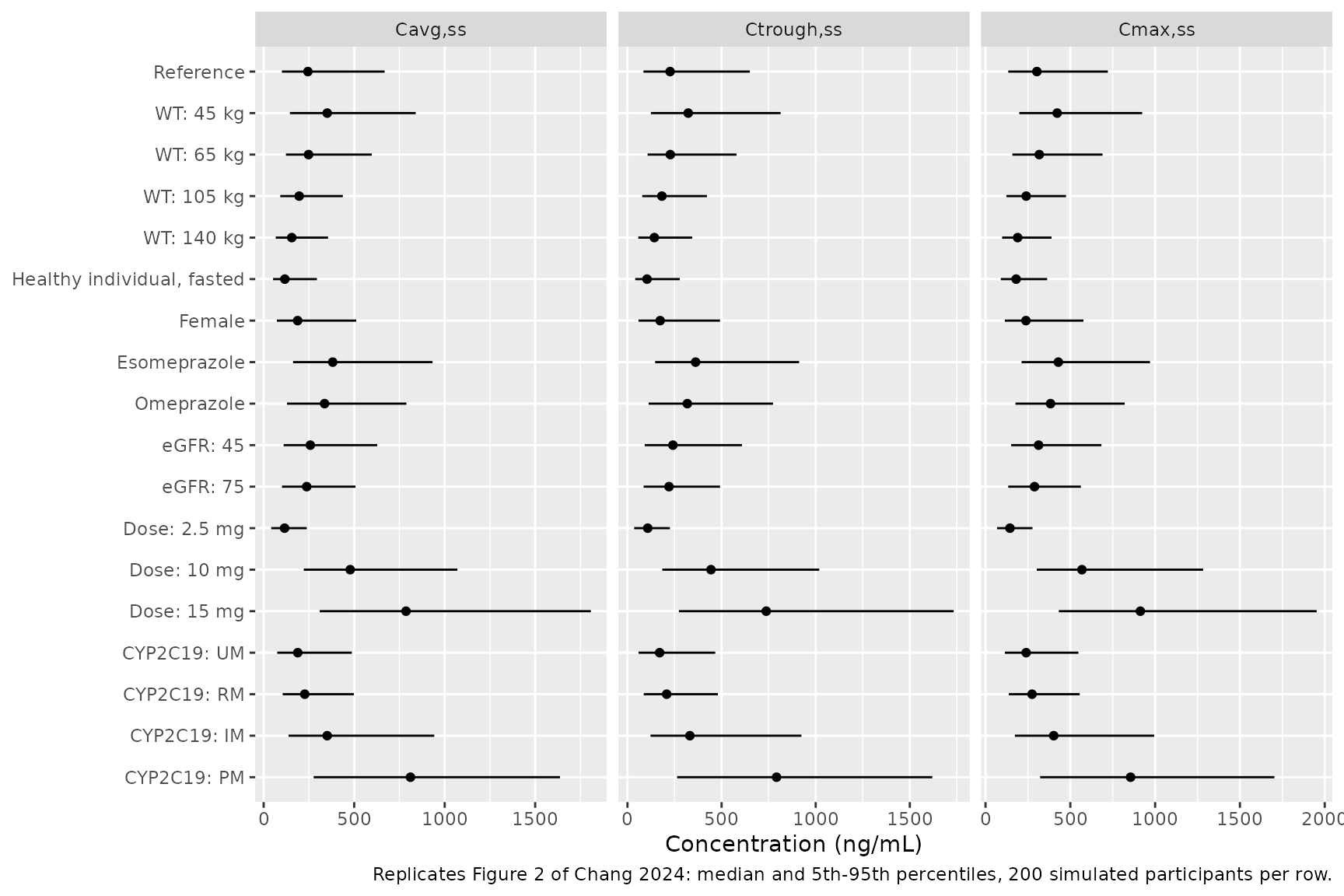
Comparison against Figure 2
The medians of Figure 2 panel (a) were digitised by the maintainers from the published figure (axis 0-2000 ng/mL over about 157 pixels, so roughly 13 ng/mL per pixel). The table compares them with the simulated medians.
published_cav <- tibble::tribble(
  ~scenario,                     ~cav,
  "Reference",                    229,
  "WT: 45 kg",                    362,
  "WT: 65 kg",                    273,
  "WT: 105 kg",                   184,
  "WT: 140 kg",                   153,
  "Healthy individual, fasted",    83,
  "Female",                       210,
  "Esomeprazole",                 388,
  "Omeprazole",                   337,
  "eGFR: 45",                     261,
  "eGFR: 75",                     242,
  "Dose: 2.5 mg",                 102,
  "Dose: 10 mg",                  502,
  "Dose: 15 mg",                  795,
  "CYP2C19: UM",                  178,
  "CYP2C19: RM",                  229,
  "CYP2C19: IM",                  343,
  "CYP2C19: PM",                  808
) |>
  mutate(scenario = factor(scenario, levels = levels(scenarios$scenario)))

cmp <- nlmixr2lib::ncaComparisonTable(
  simulated = nca_res,
  reference = published_cav,
  by = "scenario",
  params = "cav",
  units = c(cav = "ng/mL"),
  tolerance_pct = 20
)
knitr::kable(cmp, caption = "Simulated vs. digitised Figure 2(a) median Cavg,ss. * differs from the figure by more than 20%.")| NCA parameter | scenario | Reference | Simulated | % diff |
|---|---|---|---|---|
| Cavg (ng/mL) | Reference | 229 | 244 | +6.7% |
| Cavg (ng/mL) | WT: 45 kg | 362 | 351 | -3.0% |
| Cavg (ng/mL) | WT: 65 kg | 273 | 248 | -9.1% |
| Cavg (ng/mL) | WT: 105 kg | 184 | 196 | +6.6% |
| Cavg (ng/mL) | WT: 140 kg | 153 | 155 | +1.5% |
| Cavg (ng/mL) | Healthy individual, fasted | 83 | 117 | +41.0%* |
| Cavg (ng/mL) | Female | 210 | 188 | -10.6% |
| Cavg (ng/mL) | Esomeprazole | 388 | 381 | -1.7% |
| Cavg (ng/mL) | Omeprazole | 337 | 337 | -0.1% |
| Cavg (ng/mL) | eGFR: 45 | 261 | 258 | -1.2% |
| Cavg (ng/mL) | eGFR: 75 | 242 | 238 | -1.7% |
| Cavg (ng/mL) | Dose: 2.5 mg | 102 | 116 | +13.4% |
| Cavg (ng/mL) | Dose: 10 mg | 502 | 478 | -4.7% |
| Cavg (ng/mL) | Dose: 15 mg | 795 | 786 | -1.1% |
| Cavg (ng/mL) | CYP2C19: UM | 178 | 188 | +5.9% |
| Cavg (ng/mL) | CYP2C19: RM | 229 | 227 | -0.9% |
| Cavg (ng/mL) | CYP2C19: IM | 343 | 351 | +2.3% |
| Cavg (ng/mL) | CYP2C19: PM | 808 | 811 | +0.4% |
Typical-value check
With the random effects removed, Cavg,ss for each scenario must equal
F * dose / (CL/F * 24 h), written here from Table S5 values
rather than from the model file.
sim_typ <- rxode2::rxSolve(rxode2::zeroRe(mod),
  events = events_ss |> filter(id %in% seq(1, nrow(subjects), by = n_per_scenario)),
  keep = c("scenario")
) |>
  as.data.frame()
#> ℹ parameter labels from comments will be replaced by 'label()'
#> Warning: No sigma parameters in the model
#> ℹ omega/sigma items treated as zero: 'etalcl', 'etalvc', 'etalvp', 'etalka', 'etalq', 'etaruv'
#> Warning: multi-subject simulation without without 'omega'

typ <- sim_typ |>
  group_by(id, scenario) |>
  summarise(cav_sim = sum(diff(time) * (head(Cc, -1) + tail(Cc, -1)) / 2) / 24, .groups = "drop") |>
  left_join(scenarios, by = "scenario") |>
  mutate(
    cl = 0.914 * (WT / 84)^0.75 * (CRCL / 95)^0.205 *
      (1 - 0.722)^CYP2C19_PM * (1 - 0.331)^CYP2C19_IM * (1 - 0.00218)^CYP2C19_RM *
      (1 + 0.253)^CYP2C19_UM * (1 + 0.272)^DIS_HEALTHY *
      (1 - 0.332)^CONMED_OMEPRAZOLE * (1 - 0.421)^CONMED_ESOMEPRAZOLE * (1 + 0.273)^SEXF,
    f = (dose / 5)^0.0777 * (1 - 0.314)^DIS_HEALTHY * (1 + 0.0945)^SEXF,
    cav_closed = 1000 * f * dose / (cl * 24),
    pct_diff = 100 * (cav_sim / cav_closed - 1)
  )

typ |>
  select(scenario, cav_closed, cav_sim, pct_diff) |>
  mutate(across(c(cav_closed, cav_sim), \(x) signif(x, 4)), pct_diff = round(pct_diff, 2)) |>
  rename(
    "Scenario" = scenario,
    "Closed form Cavg,ss (ng/mL)" = cav_closed,
    "Simulated Cavg,ss (ng/mL)" = cav_sim,
    "Difference (%)" = pct_diff
  ) |>
knitr::kable(caption = "Typical-participant Cavg,ss: simulation against the closed form.")| Scenario | Closed form Cavg,ss (ng/mL) | Simulated Cavg,ss (ng/mL) | Difference (%) |
|---|---|---|---|
| Reference | 227.9 | 228.1 | 0.09 |
| WT: 45 kg | 364.0 | 364.3 | 0.09 |
| WT: 65 kg | 276.3 | 276.5 | 0.09 |
| WT: 105 kg | 192.8 | 193.0 | 0.09 |
| WT: 140 kg | 155.4 | 155.5 | 0.09 |
| Healthy individual, fasted | 122.9 | 123.1 | 0.14 |
| Female | 196.0 | 196.2 | 0.11 |
| Esomeprazole | 393.7 | 393.9 | 0.05 |
| Omeprazole | 341.2 | 341.4 | 0.06 |
| eGFR: 45 | 265.7 | 265.9 | 0.08 |
| eGFR: 75 | 239.3 | 239.5 | 0.08 |
| Dose: 2.5 mg | 108.0 | 108.1 | 0.09 |
| Dose: 10 mg | 481.1 | 481.5 | 0.08 |
| Dose: 15 mg | 744.7 | 745.3 | 0.08 |
| CYP2C19: UM | 181.9 | 182.1 | 0.11 |
| CYP2C19: RM | 228.4 | 228.6 | 0.09 |
| CYP2C19: IM | 340.7 | 340.9 | 0.06 |
| CYP2C19: PM | 819.9 | 820.1 | 0.02 |
# Same parameters on both sides: the only difference is trapezoidal error over
# the 17-point grid, well under 1% for this slowly varying profile.
stopifnot(all(abs(typ$pct_diff) < 1))
The typical-value Cavg,ss for the reference participant is 228 ng/mL, against about 229 ng/mL read from Figure 2.
Gate against Figure 2
The figure’s medians come from 500 simulated participants per row, so each carries about 4% sampling error on top of the digitising error. The typical-participant Cavg,ss above is the population median of Cavg,ss (no random effect enters F or the dose, and CL/F is log-normal), so it is compared with the figure directly; the 200-subject simulated medians get a looser envelope.
gate <- typ |>
  select(scenario, cav_closed) |>
  left_join(nca_ss |> group_by(scenario) |> summarise(sim = median(cav), .groups = "drop"),
    by = "scenario") |>
  left_join(published_cav, by = "scenario") |>
  mutate(
    closed_pct = 100 * (cav_closed / cav - 1),
    sim_pct = 100 * (sim / cav - 1)
  )

gate |>
  mutate(across(c(cav_closed, sim), \(x) signif(x, 3)), across(c(closed_pct, sim_pct), \(x) round(x, 1))) |>
  rename(
    "Scenario" = scenario,
    "Typical Cavg,ss (ng/mL)" = cav_closed,
    "Simulated median (ng/mL)" = sim,
    "Figure 2(a) median (ng/mL)" = cav,
    "Typical vs figure (%)" = closed_pct,
    "Simulated vs figure (%)" = sim_pct
  ) |>
knitr::kable(caption = "Median Cavg,ss against the digitised Figure 2(a).")| Scenario | Typical Cavg,ss (ng/mL) | Simulated median (ng/mL) | Figure 2(a) median (ng/mL) | Typical vs figure (%) | Simulated vs figure (%) |
|---|---|---|---|---|---|
| Reference | 228 | 244 | 229 | -0.5 | 6.7 |
| WT: 45 kg | 364 | 351 | 362 | 0.6 | -3.0 |
| WT: 65 kg | 276 | 248 | 273 | 1.2 | -9.1 |
| WT: 105 kg | 193 | 196 | 184 | 4.8 | 6.6 |
| WT: 140 kg | 155 | 155 | 153 | 1.6 | 1.5 |
| Healthy individual, fasted | 123 | 117 | 83 | 48.1 | 41.0 |
| Female | 196 | 188 | 210 | -6.7 | -10.6 |
| Esomeprazole | 394 | 381 | 388 | 1.5 | -1.7 |
| Omeprazole | 341 | 337 | 337 | 1.3 | -0.1 |
| eGFR: 45 | 266 | 258 | 261 | 1.8 | -1.2 |
| eGFR: 75 | 239 | 238 | 242 | -1.1 | -1.7 |
| Dose: 2.5 mg | 108 | 116 | 102 | 5.9 | 13.4 |
| Dose: 10 mg | 481 | 478 | 502 | -4.2 | -4.7 |
| Dose: 15 mg | 745 | 786 | 795 | -6.3 | -1.1 |
| CYP2C19: UM | 182 | 188 | 178 | 2.2 | 5.9 |
| CYP2C19: RM | 228 | 227 | 229 | -0.2 | -0.9 |
| CYP2C19: IM | 341 | 351 | 343 | -0.7 | 2.3 |
| CYP2C19: PM | 820 | 811 | 808 | 1.5 | 0.4 |
# The healthy-fasted row is the known deviation discussed below.
ok <- gate |> filter(scenario != "Healthy individual, fasted")
stopifnot(
  # Deterministic: no simulation noise on the model side. Observed spread is
  # -6.7% to +5.9%, from the figure's own sampling and digitising error;
  # dropping or sign-flipping any CYP2C19 (other than RM), PPI, weight or sex
  # effect moves its row by more than 10%.
  abs(median(ok$closed_pct)) < 3,
  all(abs(ok$closed_pct) < 10),
  # Stochastic: a 200-subject median adds about 5% sampling error per row.
  abs(median(ok$sim_pct)) < 6,
  quantile(abs(ok$sim_pct), 0.9) < 20
)
Single doses in healthy participants (Figure S1)
Supplementary Figure S1 shows mean concentrations after single oral-solution doses of 1-48 mg in fasted healthy participants (study MYK-461-002). The plot below simulates the same doses with the packaged model for a male healthy participant of 72.7 kg (the healthy-cohort mean in Table 2), eGFR 106 mL/min/1.73 m^2, CYP2C19 normal metabolizer.
sad_doses <- c(1, 2, 6, 12, 24, 48)
sad_times <- c(0.25, 0.5, 1, 1.5, 2, 3, 4, 6, 8, 12, 24, 48, 72, 96, 168, 240, 336, 504, 672)
sad <- tidyr::expand_grid(dose = sad_doses, rep = seq_len(100)) |>
  mutate(id = seq_len(n()))
sad_events <- bind_rows(
  sad |> mutate(time = 0, evid = 1L, amt = dose, cmt = "depot"),
  sad |> tidyr::expand_grid(time = sad_times) |> mutate(evid = 0L, amt = 0, cmt = "central")
) |>
  mutate(
    DOSE_MAVACAMTEN_MG = dose, WT = 72.7, CRCL = 106, SEXF = 0, DIS_HEALTHY = 1,
    FED = 0, FORM_SOLUTION = 1, CYP2C19_PM = 0, CYP2C19_IM = 0, CYP2C19_RM = 0,
    CYP2C19_UM = 0, CYP2C19_MISSING = 0, CONMED_OMEPRAZOLE = 0,
    CONMED_ESOMEPRAZOLE = 0, STUDY_MYK461014 = 0,
    treatment = paste(dose, "mg")
  ) |>
  select(id, time, evid, amt, cmt, everything(), -rep, -dose) |>
  arrange(id, time, desc(evid)) |>
  as.data.frame()

rxode2::rxSetSeed(20241030)
sim_sad <- rxode2::rxSolve(mod, events = sad_events, keep = c("treatment")) |>
  as.data.frame() |>
  mutate(treatment = factor(treatment, paste(sad_doses, "mg")))

sim_sad |>
  group_by(treatment, time) |>
  summarise(mean_Cc = mean(Cc), .groups = "drop") |>
  ggplot(aes(time, mean_Cc, colour = treatment)) +
  geom_line() +
  geom_point(size = 0.8) +
  scale_y_log10() +
  labs(x = "Time after dose (h)", y = "Mean mavacamten (ng/mL)", colour = "Dose",
    caption = "Compare with Supplementary Figure S1 of Chang 2024 (observed means, MYK-461-002).")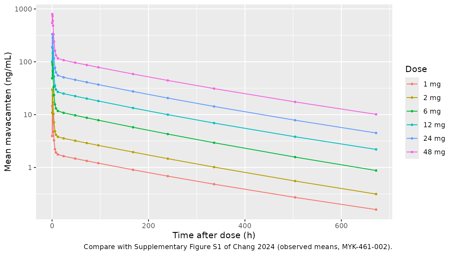
The simulated means rise and fall with the same shape as Figure S1 (a rapid peak within about 1 h, a distribution phase over the first day and a terminal phase lasting weeks). Figure S1 is a plot of observed means from six participants per dose, which are not dose-proportional at the lowest doses, so no numeric gate is placed on it. The level is informative all the same: at 48 h the simulated mean after 48 mg is 96 ng/mL, against about 95 ng/mL in Figure S1. These are fasted healthy participants, so their exposure carries the healthy-fasted F and CL/F effects of Table S5; the healthy-fasted ratio printed in Figure 2 (see below) would put them about a third lower.
Assumptions and deviations
- IIV. Table S5 reports the random effects as CV% = 100 sqrt(exp(omega^2) - 1); the packaged variances are omega^2 = log(1 + CV^2). The FDA review’s Table 4-2 reports the same model’s eta standard deviations (53.2%, 131.9%, 22.6%, 41.1%, 23% and 46.6% for CL/F, V2/F, V3/F, KA, Q/F and the residual magnitude), which are the square roots of these variances to three figures. Covariances are r omega_i * omega_j from the correlations in Table S5.
-
Residual error. The data were log-transformed. The
maintainers read Table S5 ‘EP’ (0.0292) and ‘EP14’ (0.478, study
MYK-461-014) as NONMEM SIGMA variances, so the log-scale SDs are 0.171
and 0.691. Read as SDs, 0.0292 would be a 2.9% residual error for pooled
phase 1-3 data with mainly trough sampling, which is implausibly small.
The participant-level IIV on the residual magnitude (CV 49.3%)
multiplies the SD, as an
EPS * EXP(ETA)construction would.STUDY_MYK461014should be 0 for new simulations. - Covariate reference values. Figure S2 centres continuous covariates on “the approximate median” without listing it; the maintainers used the reference participant’s values (84 kg, eGFR 95 mL/min/1.73 m^2, 5 mg), which Table 3 calls the reference for the structural estimates and which reproduce every Figure 1 percentage above.
- V3/F weight exponent. Table S5 and the FDA review list a single estimated exponent 0.813 for “Vx/F” (V2/F and V3/F). Figure 1 prints the V3/F weight effect as 75.7% and 121% with a zero-width interval, the values of the fixed 0.75 exponent used for CL/F and Q/F. The model follows the two tables.
- Food effect on KA. The Results text says KA was faster under fed than under fasted conditions, but Table S5 (and the FDA review) give an effect of +87.3% on KA for healthy fasted participants and Figure 1 plots it as 187% of the reference; the fed-healthy KA effect was removed from the final model. The model follows the table and figure.
-
Food status in patients. Food status was unknown
for every patient record, so the fed and fasted effects on KA and F
apply only when
DIS_HEALTHY = 1; patients take the reference absorption whateverFEDholds. -
CYP2C19 groups. The paper’s IM effect was estimated
in the
*1/*2-type group (Figure 1, n = 89, printed as “EM” in Tables 2 and S2). The Results report no difference in CL/F between*2/*17and*1/*2, so*2/*17carriers (n = 23) are coded IM; Figure 1 does not say where they were placed. UM is*17/*17only and RM is*1/*17. -
Dose covariate.
DOSE_MAVACAMTEN_MGis the amount of each administration (equal to the daily dose in the once-daily regimens that dominate the data). It must be set on dose records; the source carried each dose record’s value forward to the following observations. - Figure 2 deviation. The healthy-fasted row of Figure 2 is not reproduced. Its median Cavg,ss reads about 83 ng/mL (36% of the reference), but Table S5 gives F x 0.686 and CL/F x 1.272 for a healthy fasted participant, a ratio of 0.54 (123 ng/mL), which matches the text’s statement that CL/F is about 85% higher in healthy fasted participants than in patients and the FDA review’s table. The figure’s value is close to what applying the fasted-F factor twice would give (0.686^2 / 1.272 = 0.37), but the maintainers could not confirm what the figure’s simulation did. The model keeps the tabulated estimates. The other 17 rows agree within the figure’s sampling and digitising error; the FDA review’s “3.6-fold with 15 mg QD” compares with 3.27-fold from Table S5 (F rises with dose by the exponent 0.0777, which the Figure 1 F percentages at 1 and 25 mg confirm), a gap within the sampling error of a ratio of two 500-participant medians.
- No erratum for Chang 2024 was found on Europe PMC or the journal site (checked 2026-10-31).