Vincristine (van de Velde 2020)
Source:vignettes/articles/vandeVelde_2020_vincristine.Rmd
vandeVelde_2020_vincristine.RmdModel and source
- Citation: van de Velde ME, Panetta JC, Wilhelm AJ, van den Berg MH, van der Sluis IM, van den Bos C, Abbink FCH, van den Heuvel-Eibrink MM, Segers H, Chantrain C, van der Werff Ten Bosch J, Willems L, Evans WE, Kaspers GJL. Population Pharmacokinetics of Vincristine Related to Infusion Duration and Peripheral Neuropathy in Pediatric Oncology Patients. Cancers (Basel). 2020;12(7):1789. doi:10.3390/cancers12071789
- Description: Two-compartment population PK model for intravenous vincristine in children with cancer (van de Velde 2020), with body-surface-area-normalised parameters and an administration-method covariate: intercompartmental clearance and peripheral volume are each exp(1.13) = 3.1-fold higher after a push injection (1-5 min, 15-min infusions pooled) than after a 1-h infusion, while clearance and central volume do not depend on administration method.
- Article: Cancers (Basel) 2020;12(7):1789 (open access)
The paper compares vincristine given as an intravenous push injection
with the same dose given as a 1 h infusion, in children with cancer. A
linear two-compartment model was fitted in Monolix 5.1.0 (SAEM).
Administration method entered as
PK = PKpop * exp(beta * push) and was retained on the
intercompartmental clearance (IC-Cl) and the peripheral volume (V2),
each exp(1.13) = 3.1-fold higher after a push. Clearance
and central volume do not depend on administration method. So
AUC(0, inf) = Dose / CL is the same for both administration
methods, while plasma Cmax is more than twice as high after a push.
Population
Thirty-five children and adolescents took part in the PK substudy (Table 1): 20 in the push group and 15 in the 1 h infusion group. They were drawn from 90 patients in a randomized trial (Dutch Trial Registry NL4019) run at four Dutch and three Belgian centres. Mean age was 10.06 years (SD 5.6), 54% were female and 86% Caucasian. Diagnoses were acute lymphoblastic leukemia (74%), Hodgkin lymphoma (17%), and medulloblastoma, low-grade glioma or Wilms tumor (3% each). Vincristine was given at 1.5 or 2 mg/m^2 with a 2 mg maximum. The cap applied in 20 patients (37 occasions). There were 70 PK occasions (1-5 per patient) and 425 samples at 10, 20, 30, 40, 60, 75, 140 and 1440 min after the start of administration.
The same information is available programmatically via
readModelDb("vandeVelde_2020_vincristine")()$population.
Source trace
| Equation / parameter | Value | Source location |
|---|---|---|
lcl (CL per m^2) |
log(30.5) L/h/m^2 | Table 2, Administration Type model, Cl (RSE 10.0%) |
lvc (V1 per m^2) |
log(20.8) L/m^2 | Table 2, V1 (RSE 12.5%) |
lq (IC-Cl per m^2, 1 h infusion) |
log(34.2) L/h/m^2 | Table 2, IC-Cl (RSE 9.5%) |
lvp (V2 per m^2, 1 h infusion) |
log(127.7) L/m^2 | Table 2, V2 (RSE 19.0%) |
e_push_q |
1.13 | Table 2, beta on IC-CL (push) (RSE 4.5%) |
e_push_vp |
1.13 | Table 2, beta on V2 (push) (RSE 19.1%) |
etalcl, etalvc, etalq,
etalvp
|
0.52^2, 0.55^2, 0.48^2, 0.41^2 | Table 2, inter-individual variability (Monolix omega, see Assumptions) |
propSd |
0.45 | Table 2, Residual; proportional model per Methods 4.5 |
PK = PKpop * exp(beta * push) |
n/a | Table 2 footnote |
push = 1 for 1-5 min push (15-min infusions pooled), 0
for 1 h infusion |
n/a | Methods 4.2, Results 2.1 |
| Linear 2-compartment ODE, first-order elimination | n/a | Methods 4.5, Figure 3 |
| Parameters scaled per m^2 BSA | n/a | Table 2 units, Figure 3 caption |
Typical-value profiles (Figure 1)
Figure 1 of the paper overlays the typical model fit for each
administration method on the observed concentrations over 0-3 h. The
push curve starts at about 75 ng/mL, which equals
1.5 mg/m^2 / 20.8 L/m^2. The figure is therefore drawn for
a 1.5 mg/m^2 dose, normalised to 1 m^2. The 1 h curve peaks at about 32
ng/mL near 0.7 h. The 1 h infusion was a 38-min bag followed by a 22-min
flush (Methods 4.2), and a 38-min input reproduces that peak. Both input
durations are shown.
mod <- readModelDb("vandeVelde_2020_vincristine")
mod_typ <- mod |> rxode2::zeroRe()
#> ℹ parameter labels from comments will be replaced by 'label()'

typ_grid <- sort(unique(c(seq(0, 3, by = 0.01), 1 / 60, 38 / 60)))
typ_arms <- tibble::tribble(
  ~arm,                              ~dur,
  "Push (1 min)",                    1 / 60,
  "1 h infusion (60 min input)",     1,
  "1 h infusion (38 min bag input)", 38 / 60
)

make_typ <- function(i) {
  a <- typ_arms[i, ]
  dplyr::bind_rows(
    tibble(id = i, time = 0, evid = 1L, amt = 1.5, dur = a$dur, cmt = "central"),
    tibble(id = i, time = typ_grid, evid = 0L, amt = 0, dur = 0, cmt = "central")
  ) |>
    dplyr::mutate(BSA = 1, TINF = a$dur, arm = a$arm)
}
typ_ev <- dplyr::bind_rows(lapply(seq_len(nrow(typ_arms)), make_typ))

sim_typ <- rxode2::rxSolve(mod_typ, events = typ_ev, keep = "arm") |>
  as.data.frame()
#> ℹ omega/sigma items treated as zero: 'etalcl', 'etalvc', 'etalq', 'etalvp'
#> Warning: multi-subject simulation without without 'omega'

ggplot(sim_typ, aes(time, Cc, linetype = arm)) +
  geom_line() +
  scale_y_log10(limits = c(0.1, 100)) +
  labs(
    x = "Time (h)", y = "Vincristine concentration (ng/mL)", linetype = NULL,
    title = "Typical-value profiles, 1.5 mg/m^2 at BSA 1 m^2",
    caption = "Replicates the model curves of Figure 1 of van de Velde 2020."
  ) +
  theme(legend.position = "bottom")
#> Warning in scale_y_log10(limits = c(0.1, 100)): log-10 transformation
#> introduced infinite values.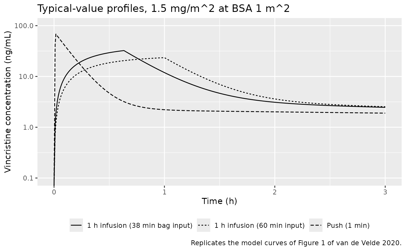
typ_summary <- sim_typ |>
  dplyr::group_by(arm) |>
  dplyr::summarise(
    cmax = max(Cc), tmax = time[which.max(Cc)],
    c_3h = Cc[time == 3], .groups = "drop"
  )
knitr::kable(typ_summary, digits = 2,
caption = "Typical-value Cmax, Tmax and 3 h concentration.")| arm | cmax | tmax | c_3h |
|---|---|---|---|
| 1 h infusion (38 min bag input) | 32.34 | 0.63 | 2.46 |
| 1 h infusion (60 min input) | 23.47 | 1.00 | 2.54 |
| Push (1 min) | 68.32 | 0.02 | 1.90 |
push_row <- typ_summary[typ_summary$arm == "Push (1 min)", ]
bag_row <- typ_summary[typ_summary$arm == "1 h infusion (38 min bag input)", ]
stopifnot(
  # Push peak is Dose / V1 less the loss over the 1-min input; Figure 1 reads ~75
  push_row$cmax > 60, push_row$cmax < 75,
  # Figure 1: the push curve has flattened to ~2 ng/mL by 3 h
  push_row$c_3h > 1.5, push_row$c_3h < 2.5,
  # Figure 1: the 1 h curve peaks at ~32 ng/mL near 0.7 h and is ~3 ng/mL at 3 h
  bag_row$cmax > 28, bag_row$cmax < 36,
  bag_row$c_3h > 2, bag_row$c_3h < 3.5
)
Administration method does not change AUC(0, inf)
In a linear model AUC(0, inf) = Dose / CL regardless of
how the dose is put in, and administration method does not act on CL
here. The paper reports the same thing: plasma AUC did not differ
significantly between the groups (Table 3). The check below solves the
typical subject to 400 h on a log-spaced grid. It confirms that both
administration methods return Dose / CL. The check compares
a solve with its own closed form, so a tight bound is appropriate.
long_grid <- sort(unique(c(0, 10^seq(-3, log10(400), length.out = 3000), 1 / 60, 1)))
inv_ev <- dplyr::bind_rows(lapply(1:2, function(i) {
  d <- c(1 / 60, 1)[i]
  dplyr::bind_rows(
    tibble(id = i, time = 0, evid = 1L, amt = 1.5, dur = d, cmt = "central"),
    tibble(id = i, time = long_grid, evid = 0L, amt = 0, dur = 0, cmt = "central")
  ) |>
    dplyr::mutate(BSA = 1, TINF = d, arm = c("Push", "1 h infusion")[i])
}))
sim_inv <- rxode2::rxSolve(mod_typ, events = inv_ev, keep = "arm") |>
  as.data.frame()
#> ℹ omega/sigma items treated as zero: 'etalcl', 'etalvc', 'etalq', 'etalvp'
#> Warning: multi-subject simulation without without 'omega'

trap <- function(t, y) sum(diff(t) * (head(y, -1) + tail(y, -1)) / 2)
auc_inv <- sim_inv |>
  dplyr::group_by(arm) |>
  dplyr::summarise(
    auc_0_400 = trap(time, Cc),
    dose_over_cl = 1.5 / cl[1] * 1000,
    q = q[1], vp = vp[1],
    .groups = "drop"
  ) |>
  dplyr::mutate(rel_err = auc_0_400 / dose_over_cl - 1)
knitr::kable(auc_inv, digits = c(0, 2, 2, 1, 1, 4))| arm | auc_0_400 | dose_over_cl | q | vp | rel_err |
|---|---|---|---|---|---|
| 1 h infusion | 49.18 | 49.18 | 34.2 | 127.7 | 0 |
| Push | 49.18 | 49.18 | 105.9 | 395.3 | 0 |
stopifnot(
  all(abs(auc_inv$rel_err) < 0.01),
  # push multiplies q and vp by exp(1.13) = 3.096 (Results 2.2: '3.1 times higher')
  abs(auc_inv$q[auc_inv$arm == "Push"] / auc_inv$q[auc_inv$arm == "1 h infusion"] - exp(1.13)) < 1e-6,
  abs(auc_inv$vp[auc_inv$arm == "Push"] / auc_inv$vp[auc_inv$arm == "1 h infusion"] - exp(1.13)) < 1e-6
)
Virtual cohort
The observed data are not public. The cohort below approximates Table
1. Age is drawn from a normal distribution with mean 10.06 and SD 5.6
years, truncated to 1-18 years. Weight and height come from sex-averaged
50th-percentile growth values with log-normal scatter, and BSA from the
Mosteller formula. Each subject gets 1.5 or 2 mg/m^2 with equal
probability, capped at 2 mg (Methods 4.2). The paper does not report the
split between the two dose levels. A push is given over 3 min, the
middle of the 1-5 min definition. For a 1 h infusion the drug goes in
over 38 min, the length of the drug-containing bag; the remaining 22 min
flush the line (Methods 4.2). Its TINF is still the nominal
1 h, so the administration-method covariate is unchanged. Figure 1 and
the Table 3 plasma Cmax both support the 38-min input (see Assumptions).
There are 100 subjects per arm and one occasion each.
set.seed(20200704)
rxode2::rxSetSeed(20200704)
n_per_arm <- 100L

growth <- tibble::tribble(
  ~age, ~wt,  ~ht,
  1,    9.9,  75,
  2,    12.5, 87,
  4,    16.3, 103,
  6,    20.7, 116,
  8,    25.6, 128,
  10,   32.0, 138,
  12,   40.5, 150,
  14,   50.0, 162,
  16,   58.0, 170,
  18,   63.0, 172
)

draw_age <- function(n) {
  out <- numeric(0)
  while (length(out) < n) {
    x <- rnorm(n, 10.06, 5.6)
    out <- c(out, x[x >= 1 & x <= 18])
  }
  out[seq_len(n)]
}

obs_times <- sort(unique(c(
  0, seq(0.025, 3, by = 0.025), seq(3.25, 24, by = 0.25), 3 / 60, 38 / 60, 1
)))

make_arm <- function(n, arm, tinf, input_dur, id_offset) {
  subj <- tibble(
    id = id_offset + seq_len(n),
    age = draw_age(n)
  ) |>
    dplyr::mutate(
      WT = approx(growth$age, growth$wt, age)$y * exp(rnorm(n, 0, 0.15)),
      HT = approx(growth$age, growth$ht, age)$y * exp(rnorm(n, 0, 0.04)),
      BSA = sqrt(WT * HT / 3600),
      dose_m2 = sample(c(1.5, 2), n, replace = TRUE),
      amt_mg = pmin(dose_m2 * BSA, 2),
      capped = dose_m2 * BSA > 2,
      arm = arm, TINF = tinf, input_dur = input_dur
    )
  doses <- subj |>
    dplyr::transmute(id, time = 0, evid = 1L, amt = amt_mg, dur = input_dur,
                     cmt = "central", BSA, TINF, arm)
  obs <- subj |>
    dplyr::select(id, BSA, TINF, arm) |>
    tidyr::crossing(time = obs_times) |>
    dplyr::mutate(evid = 0L, amt = 0, dur = 0, cmt = "central")
  list(subj = subj, events = dplyr::bind_rows(doses, obs) |> dplyr::arrange(id, time, dplyr::desc(evid)))
}

arm_push <- make_arm(n_per_arm, "Push", tinf = 3 / 60, input_dur = 3 / 60, id_offset = 0L)
arm_1h <- make_arm(n_per_arm, "1 h infusion", tinf = 1, input_dur = 38 / 60, id_offset = n_per_arm)
subjects <- dplyr::bind_rows(arm_push$subj, arm_1h$subj)
events <- dplyr::bind_rows(arm_push$events, arm_1h$events)
stopifnot(!anyDuplicated(unique(events[, c("id", "time", "evid")])))

subjects |>
  dplyr::group_by(arm) |>
  dplyr::summarise(
    n = dplyr::n(), mean_age = mean(age), median_BSA = median(BSA),
    pct_capped = 100 * mean(capped), .groups = "drop"
  ) |>
knitr::kable(digits = 2, caption = "Virtual cohort summary.")| arm | n | mean_age | median_BSA | pct_capped |
|---|---|---|---|---|
| 1 h infusion | 100 | 10.49 | 1.21 | 52 |
| Push | 100 | 10.26 | 1.13 | 53 |
Simulation
sim <- rxode2::rxSolve(mod, events = events, keep = "arm") |>
  as.data.frame() |>
  dplyr::mutate(Cp = peripheral1 / vp * 1000)
#> ℹ parameter labels from comments will be replaced by 'label()'
sim |>
  dplyr::filter(time <= 3) |>
  dplyr::group_by(arm, time) |>
  dplyr::summarise(
    Q05 = quantile(Cc, 0.05), Q50 = median(Cc), Q95 = quantile(Cc, 0.95),
    .groups = "drop"
  ) |>
  ggplot(aes(time, Q50)) +
  geom_ribbon(aes(ymin = Q05, ymax = Q95), alpha = 0.25) +
  geom_line() +
  facet_wrap(~arm) +
  scale_y_log10() +
  labs(x = "Time (h)", y = "Vincristine concentration (ng/mL)",
       title = "Simulated median and 90% interval, 0-3 h",
       caption = "Compare with the observed data in Figure 1 of van de Velde 2020.")
#> Warning in scale_y_log10(): log-10 transformation introduced infinite values.
#> log-10 transformation introduced infinite values.
#> log-10 transformation introduced infinite values.
#> log-10 transformation introduced infinite values.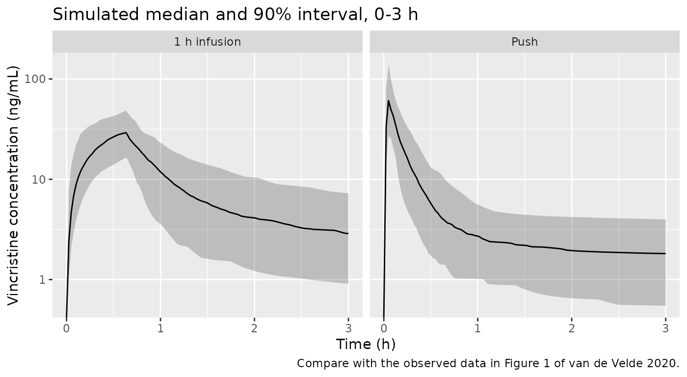
PKNCA validation
Table 3 of the paper gives medians of the post-hoc plasma and peripheral AUC and Cmax for each administration method. The Methods call the AUC window “0-3 h”, but the published values match a 0-24 h window, the paper’s sampling horizon (see Assumptions). The NCA below therefore uses 0-24 h. The peripheral “concentration” is the peripheral amount divided by V2, as in the paper, and gets its own PKNCA block.
dose_df <- events |>
  dplyr::filter(evid == 1) |>
  dplyr::select(id, time, amt, arm)
dose_obj <- PKNCA::PKNCAdose(dose_df, amt ~ time | arm + id)
intervals <- data.frame(start = 0, end = 24, cmax = TRUE, auclast = TRUE)

run_nca <- function(conc_col) {
  d <- sim |>
    dplyr::transmute(id, time, conc = .data[[conc_col]], arm) |>
    dplyr::filter(!is.na(conc))
  conc_obj <- PKNCA::PKNCAconc(d, conc ~ time | arm + id)
  PKNCA::pk.nca(PKNCA::PKNCAdata(conc_obj, dose_obj, intervals = intervals))
}
nca_plasma <- run_nca("Cc")
nca_periph <- run_nca("Cp")
Comparison against published post-hoc exposures (Table 3)
pub_plasma <- tibble::tribble(
  ~arm,           ~cmax, ~auclast,
  "1 h infusion", 30.05, 44.04,
  "Push",         72.44, 38.60
)
pub_periph <- tibble::tribble(
  ~arm,           ~cmax, ~auclast,
  "1 h infusion", 4.81,  42.50,
  "Push",         2.57,  35.36
)
nca_units <- c(cmax = "ng/mL", auclast = "ng*h/mL")

cmp_plasma <- nlmixr2lib::ncaComparisonTable(
  simulated = nca_plasma, reference = pub_plasma, by = "arm",
  units = nca_units, tolerance_pct = 20
)
knitr::kable(cmp_plasma, caption = "Plasma: simulated vs. published median (Table 3). * differs by >20%.")| NCA parameter | arm | Reference | Simulated | % diff |
|---|---|---|---|---|
| Cmax (ng/mL) | 1 h infusion | 30 | 29.2 | -3.0% |
| Cmax (ng/mL) | Push | 72.4 | 61 | -15.8% |
| AUClast (ng*h/mL) | 1 h infusion | 44 | 49 | +11.2% |
| AUClast (ng*h/mL) | Push | 38.6 | 39 | +0.9% |
cmp_periph <- nlmixr2lib::ncaComparisonTable(
  simulated = nca_periph, reference = pub_periph, by = "arm",
  units = nca_units, tolerance_pct = 20
)
knitr::kable(cmp_periph, caption = "Peripheral compartment: simulated vs. published median (Table 3). * differs by >20%.")| NCA parameter | arm | Reference | Simulated | % diff |
|---|---|---|---|---|
| Cmax (ng/mL) | 1 h infusion | 4.81 | 5.72 | +19.0% |
| Cmax (ng/mL) | Push | 2.57 | 2.62 | +1.8% |
| AUClast (ng*h/mL) | 1 h infusion | 42.5 | 46.3 | +8.9% |
| AUClast (ng*h/mL) | Push | 35.4 | 34.9 | -1.4% |
sim_medians <- function(res) {
  as.data.frame(res$result) |>
    dplyr::filter(PPTESTCD %in% c("cmax", "auclast")) |>
    dplyr::group_by(arm, PPTESTCD) |>
    dplyr::summarise(sim = median(PPORRES), .groups = "drop")
}
gate <- dplyr::bind_rows(
  sim_medians(nca_plasma) |>
    dplyr::inner_join(tidyr::pivot_longer(pub_plasma, -arm, names_to = "PPTESTCD", values_to = "pub"),
                      by = c("arm", "PPTESTCD")) |>
    dplyr::mutate(matrix = "plasma"),
  sim_medians(nca_periph) |>
    dplyr::inner_join(tidyr::pivot_longer(pub_periph, -arm, names_to = "PPTESTCD", values_to = "pub"),
                      by = c("arm", "PPTESTCD")) |>
    dplyr::mutate(matrix = "peripheral")
) |>
  dplyr::mutate(ratio = sim / pub)
knitr::kable(gate, digits = 3, caption = "Simulated / published median ratios.")| arm | PPTESTCD | sim | pub | matrix | ratio |
|---|---|---|---|---|---|
| 1 h infusion | auclast | 48.971 | 44.04 | plasma | 1.112 |
| 1 h infusion | cmax | 29.162 | 30.05 | plasma | 0.970 |
| Push | auclast | 38.958 | 38.60 | plasma | 1.009 |
| Push | cmax | 60.995 | 72.44 | plasma | 0.842 |
| 1 h infusion | auclast | 46.297 | 42.50 | peripheral | 1.089 |
| 1 h infusion | cmax | 5.725 | 4.81 | peripheral | 1.190 |
| Push | auclast | 34.868 | 35.36 | peripheral | 0.986 |
| Push | cmax | 2.617 | 2.57 | peripheral | 1.018 |
# Medians of 100 simulated subjects per arm. A wrong clearance, volume, push
# multiplier, dose or unit (e.g. a missing mg -> ng/mL factor) moves these by
# a factor of 1.5 or more. The +/-30% envelope absorbs cohort-to-cohort
# variation and the unreported dose-level split. Across three cohort seeds the
# eight ratios spanned 0.81-1.21, so do not tighten this without re-measuring.
stopifnot(all(gate$ratio > 0.7 & gate$ratio < 1.3))

# Direction of the administration-method effect (Table 3): plasma Cmax more
# than 2-fold higher and peripheral Cmax about 2-fold lower after a push.
pc <- function(m, a) gate$sim[gate$matrix == m & gate$arm == a & gate$PPTESTCD == "cmax"]
stopifnot(
  pc("plasma", "Push") / pc("plasma", "1 h infusion") > 1.6,
  pc("peripheral", "1 h infusion") / pc("peripheral", "Push") > 1.4
)
Time above 1 ng/mL
Results 2.2 gives median times above 1 ng/mL. For the peripheral compartment these are 14.65 h (1 h infusion) and 16.83 h (push). For plasma they are 0.92 h and 0.24 h.
dt_grid <- sim |>
  dplyr::arrange(id, time) |>
  dplyr::group_by(id, arm) |>
  dplyr::mutate(dt = dplyr::lead(time) - time) |>
  dplyr::filter(!is.na(dt))
tab <- dt_grid |>
  dplyr::summarise(
    plasma_gt1 = sum(dt[Cc > 1]),
    plasma_gt10 = sum(dt[Cc > 10]),
    periph_gt1 = sum(dt[Cp > 1]),
    .groups = "drop"
  ) |>
  dplyr::group_by(arm) |>
  dplyr::summarise(dplyr::across(c(plasma_gt1, plasma_gt10, periph_gt1), median), .groups = "drop") |>
  dplyr::mutate(published_periph_gt1 = c(`1 h infusion` = 14.65, Push = 16.83)[as.character(arm)],
                published_plasma_gt1 = c(`1 h infusion` = 0.92, Push = 0.24)[as.character(arm)])
knitr::kable(tab, digits = 2, caption = "Median time (h) above the threshold within 0-24 h.")| arm | plasma_gt1 | plasma_gt10 | periph_gt1 | published_periph_gt1 | published_plasma_gt1 |
|---|---|---|---|---|---|
| 1 h infusion | 9.72 | 0.95 | 14.85 | 14.65 | 0.92 |
| Push | 13.47 | 0.35 | 18.01 | 16.83 | 0.24 |
The peripheral times match. The published plasma times (0.92 h and 0.24 h) cannot be times above 1 ng/mL. Figure 1 shows the push group still above 1 ng/mL at 3 h. The simulated time above 10 ng/mL is close to the published numbers, so the plasma threshold in the text is probably a misprint for 10 ng/mL. Neither plasma value is gated.
Assumptions and deviations
-
IIV scale. Table 2 prints the inter-individual
variability as 0.52, 0.55, 0.48 and 0.41 under a “CV%” header. These
values match Monolix’s
omegaoutput, the SD of the normally distributed log-parameter. They are encoded as variancesomega^2. If they were fractional CVs, the variances would belog(1 + CV^2), 5-12% smaller, which matters little in practice. - Inter-occasion variability. Methods 4.5 says inter-occasion variability was assumed log-normal, but Table 2 reports no IOV estimates. IOV is therefore not encoded.
-
Administration-method covariate. The paper’s binary
pushcovariate is derived from the canonical infusion-duration columnTINF. It is 1 whenTINF < 0.5h and 0 otherwise. Push injections (1-5 min), the two 15-min infusions analysed as push, and the 60- or 96-min “1 h” infusions all fall on the same side of any threshold between 0.25 h and 1 h. - AUC window. Methods 4.5 describes the post-hoc AUC as “AUC (0-3 h)”. Over 0-3 h the typical 1.5 mg/m^2 AUC is about 28 ngh/mL (1 h infusion) and 16 ngh/mL (push), roughly 35-60% below the published medians of 44.04 and 38.60 ngh/mL. Over 0-24 h it is about 47 and 39 ngh/mL, which matches, and so does the peripheral AUC. The comparison here uses 0-24 h. This follows the paper’s own exposure values; no parameter was adjusted.
- Plasma time above 1 ng/mL. See the previous section. The published plasma values look like times above 10 ng/mL and are not gated.
- Virtual cohort. The age distribution comes from Table 1 (mean 10.06, SD 5.6), truncated to 1-18 years. Weight and height are approximate sex-averaged 50th-percentile growth values with log-normal scatter, and BSA uses the Mosteller formula (the paper does not name its formula). The split between the 1.5 and 2 mg/m^2 dose levels is not reported, so it is set to 50:50. The push is given over 3 min, the midpoint of 1-5 min.
- 1 h infusion input profile. The paper does not say what infusion duration its dataset recorded. Methods 4.2 describes a 38-min bag followed by a 22-min flush of the line. The virtual cohort puts the dose in over those 38 min. The typical 38-min input peaks at 32 ng/mL near 0.63 h, matching the 1 h curve in Figure 1 (about 32 ng/mL near 0.7 h). A 60-min input peaks at 23 ng/mL at 1 h, below Figure 1 and below the Table 3 median plasma Cmax of 30.05 ng/mL. The input duration does not change AUC(0, inf). The four patients from one hospital with a 96-min administration (60-min bag) are not represented.
- Clearance difference by method. A trend towards lower CL in the push group (p = 0.058) was not retained in the final model (Results 2.2) and is not encoded.
-
Concomitant azoles. Concomitant azole antifungal
treatment was tested and was not significant. It is documented in
covariatesDataExcluded. - No correction notice for this article was found on Europe PMC as of 2026-09-27.