Ethambutol in ICU and outpatients with tuberculosis (Beraldi-Magalhaes 2021)
Source:vignettes/articles/BeraldiMagalhaes_2021_ethambutol.Rmd
BeraldiMagalhaes_2021_ethambutol.RmdModel and source
#> ℹ parameter labels from comments will be replaced by 'label()'Citation: Beraldi-Magalhaes F, Parker SL, Sanches C, Sousa Garcia L, Souza Carvalho BK, Fachi MM, de Liz MV, Pontarolo R, Lipman J, Cordeiro-Santos M, Roberts JA. Is Dosing of Ethambutol as Part of a Fixed-Dose Combination Product Optimal for Mechanically Ventilated ICU Patients with Tuberculosis? A Population Pharmacokinetic Study. Antibiotics (Basel). 2021;10(12):1559. doi:10.3390/antibiotics10121559. PMCID: PMC8698281.
Description: Two-compartment oral population PK model of ethambutol given as a crushed or whole rifampin/isoniazid/pyrazinamide/ethambutol fixed-dose-combination (FDC) tablet to 30 Brazilian adults with tuberculosis: 10 mechanically ventilated ICU patients (tablet crushed and given by nasogastric tube) and 20 outpatients (tablet swallowed whole). Fitted non-parametrically with NPAG in Pmetrics 1.5.0. Every structural parameter – clearance, central volume, first- and second-occasion absorption rate constants, bioavailability, intercompartmental clearance and peripheral volume – was estimated separately for the ICU and outpatient groups inside one model, so each carries an _icu / _outpt stratum suffix selected by DIS_CRITILL, with its own log-normal IIV approximated from the Table 3 %CV. Creatinine clearance normalised to 101 mL/min scales clearance and total body weight normalised to 56 kg scales both volumes with a 0.25 allometric exponent. Residual error is fixed(0) because the Pmetrics error-model coefficients are not published. The published ICU parameters do not reproduce the paper’s own observed ICU exposures; see the vignette.
Article: https://doi.org/10.3390/antibiotics10121559 (open access; PMCID
PMC8698281)
Beraldi-Magalhaes and colleagues compare the pharmacokinetics of
ethambutol given as part of a four-drug fixed-dose-combination (FDC)
tablet in two groups of adults with tuberculosis in Manaus, Brazil: 10
mechanically ventilated ICU patients, whose tablets were crushed and
given through a nasogastric tube, and 20 outpatients, who swallowed
whole tablets. One two-compartment model with first-order absorption was
fitted with the non-parametric NPAG algorithm in Pmetrics. Every
structural parameter was estimated separately for the two groups (“using
selective execution statements”), so the packaged model carries two full
parameter sets, selected by the DIS_CRITILL covariate (1 =
ICU, 0 = outpatient).
Read the “ICU parameter set” section before using the ICU arm. The published ICU parameters do not reproduce either the paper’s own observed ICU exposures or its own ICU target-attainment simulations. The outpatient arm does reproduce both.
Population
Thirty adults were analysed (Table 1): 10 ICU patients (median age 31 years, weight 51.2 kg, measured creatinine clearance 92.3 mL/min, SOFA 10, APACHE II 20.5, 8/10 on vasoactive drugs) and 20 outpatients (median age 39.5 years, weight 58.35 kg, creatinine clearance 113.88 mL/min). Both groups were 80% male, and HIV co-infection was common (9/10 ICU, 15/20 outpatients). All received the weight-banded FDC dose of the Brazilian guideline: 550 mg (20-35 kg), 825 mg (36-50 kg) or 1100 mg (> 50 kg) ethambutol once daily. Plasma was sampled before the dose and at 0.5, 1, 2, 4, 6, 8, 12 and 24 h on enrolment days 1 and 3, after a median of 10 (ICU) or 11 (outpatients) days of treatment, giving 352 concentrations.
| Field | Value |
|---|---|
| species | human |
| n_subjects | 30 |
| n_studies | 1 |
| age_range | Adults >= 18 years; median 31.0 (IQR 29-40) ICU, 39.5 (IQR 32.7-46.2) outpatients |
| weight_range | Median 51.2 kg (IQR 46.2-58.6) ICU, 58.35 kg (IQR 53.2-67) outpatients |
| sex_female_pct | 20 |
| race_ethnicity | Not reported (Amazonas State, Brazil) |
| disease_state | Active pulmonary or extrapulmonary tuberculosis. 10 mechanically ventilated ICU patients (median SOFA 10, APACHE II 20.5, 8/10 on vasoactive drugs) and 20 outpatients. HIV co-infection in 9/10 ICU patients and 15/20 outpatients. Measured creatinine clearance median 92.3 mL/min (ICU) and 113.88 mL/min (outpatients); patients on any form of dialysis or renal replacement therapy were excluded. |
| dose_range | Once-daily weight-banded FDC tablets (rifampin/isoniazid/pyrazinamide/ethambutol) per the Brazilian Ministry of Health guideline: 550 mg (20-35 kg), 825 mg (36-50 kg) or 1100 mg (> 50 kg) ethambutol. ICU: crushed, suspended in 20 mL water, via nasogastric tube. Outpatients: whole tablets orally, directly observed. |
| regions | Brazil (Fundacao de Medicina Tropical Dr. Heitor Vieira Dourado, Manaus, Amazonas) |
| notes | Beraldi-Magalhaes 2021 Table 1. 352 plasma concentrations; samples pre-dose and at 0.5, 1, 2, 4, 6, 8, 12 and 24 h on enrolment days 1 and 3, after a median 10 (ICU) or 11 (outpatients) days of treatment. Total ethambutol by LC-MS/MS (0.2-5 mg/L with a dilution QC). The pre-dose concentration of each subject was used as the model initial condition during fitting; that data-fitting device is not encoded here (see the vignette). |
Source trace
Every ini() entry carries an in-file comment naming its
source location. All structural values are the mean of
the NPAG marginal distribution in Table 3.
| Equation / parameter | ICU (_icu) |
Outpatients (_outpt) |
Source location |
|---|---|---|---|
lcl_* (CL at CRCL = 101 mL/min) |
1.2 L/h | 17.5 L/h | Table 3 ‘Clearance (L/h)’, mean |
lvc_* (Vc at WT = 56 kg) |
64.8 L | 137.2 L | Table 3 ‘Volume (L)’, mean |
lka_occ1_* (ka, first sampled dose) |
0.72 1/h | 0.35 1/h | Table 3 ‘Ka1 (h-1)’, mean |
lka_occ2_* (ka, second sampled dose) |
0.75 1/h | 0.39 1/h | Table 3 ‘Ka2 (h-1)’, mean |
lfdepot_* (F) |
0.80 | 0.14 | Table 3 ‘F’, mean |
lq_* (Q) |
7.3 L/h | 2.66 L/h | Table 3 ‘Q(L/h)’, mean |
lvp_* (Vp at WT = 56 kg) |
348.6 L | 343.3 L | Table 3 ‘Vp (L)’, mean |
eta*_* |
from CV% | from CV% | Table 3 %CV, as log(CV^2 + 1)
|
e_wt_vc_vp |
fixed(0.25) |
(shared) | Results 2.2: WT normalised to 56 kg, allometric scaler ‘raised to the 25th power’ on Vc and Vp |
CL * (CRCL / 101) |
(shared) | Results 2.2: ‘creatinine clearance normalized to 101 mL/min on clearance’ | |
propSd, addSd
|
fixed(0) |
fixed(0) |
Not reported (Methods 4.4 names the Pmetrics error model but not its coefficients) |
| Two compartments, first-order absorption, linear elimination | Results 2.2 | ||
ka by occasion (OCC) |
Methods 4.4; Table 3 footnote ‘absorption rate constant for the 1st and 2nd dose’ |
Table 3 prints a mean, SD, median and %CV for each parameter and
group. SD / mean reproduces the printed %CV on every row to
within the rounding of the printed SD, which is what licenses
omega^2 = log(CV^2 + 1).
tab3 <- tibble::tribble(
  ~group,        ~parameter, ~mean, ~sd,  ~median, ~cv_pct,
  "ICU",         "CL",        1.2,   1.5,   0.9,   120.9,
  "ICU",         "V",        64.8,  11.7,  61.1,    18.1,
  "ICU",         "Ka1",       0.72,  0.05,  0.7,     7.4,
  "ICU",         "Ka2",       0.75,  0.10,  0.8,    13.8,
  "ICU",         "F",         0.80,  0.06,  0.8,     7.9,
  "ICU",         "Q",         7.3,   3.5,   6.6,    48.6,
  "ICU",         "Vp",      348.6,  30.1, 361.6,     8.6,
  "Outpatients", "CL",       17.5,  13.3,  11.1,    75.8,
  "Outpatients", "V",       137.2,  55.1, 170.4,    40.1,
  "Outpatients", "Ka1",       0.35,  0.12,  0.3,    35.5,
  "Outpatients", "Ka2",       0.39,  0.18,  0.4,    44.9,
  "Outpatients", "F",         0.14,  0.13,  0.1,    87.1,
  "Outpatients", "Q",         2.66,  2.02,  3.8,    75.9,
  "Outpatients", "Vp",      343.3,  78.2, 400.0,    22.8
) |>
  dplyr::mutate(
    cv_from_sd = 100 * sd / mean,
    omega2 = log((cv_pct / 100)^2 + 1)
  )

# The printed CV% is SD/mean on the linear scale. The two largest gaps (ICU CL
# 125.0 vs 120.9, outpatient F 92.9 vs 87.1) are both inside the rounding of a
# 2-significant-figure SD over a 2-significant-figure mean.
stopifnot(abs(stats::median(tab3$cv_from_sd - tab3$cv_pct)) < 1)
stopifnot(max(abs(tab3$cv_from_sd / tab3$cv_pct - 1)) < 0.07)

tab3 |>
  dplyr::select(group, parameter, mean, sd, median, cv_pct, cv_from_sd, omega2) |>
  dplyr::rename(
    "Group" = group,
    "Parameter" = parameter,
    "Mean" = mean,
    "SD" = sd,
    "Median" = median,
    "CV% (printed)" = cv_pct,
    "100 x SD/mean" = cv_from_sd,
    "omega^2 encoded" = omega2
  ) |>
knitr::kable(digits = 4, caption = "Table 3 of Beraldi-Magalhaes 2021 with the CV% identity check.")| Group | Parameter | Mean | SD | Median | CV% (printed) | 100 x SD/mean | omega^2 encoded |
|---|---|---|---|---|---|---|---|
| ICU | CL | 1.20 | 1.50 | 0.9 | 120.9 | 125.0000 | 0.9008 |
| ICU | V | 64.80 | 11.70 | 61.1 | 18.1 | 18.0556 | 0.0322 |
| ICU | Ka1 | 0.72 | 0.05 | 0.7 | 7.4 | 6.9444 | 0.0055 |
| ICU | Ka2 | 0.75 | 0.10 | 0.8 | 13.8 | 13.3333 | 0.0189 |
| ICU | F | 0.80 | 0.06 | 0.8 | 7.9 | 7.5000 | 0.0062 |
| ICU | Q | 7.30 | 3.50 | 6.6 | 48.6 | 47.9452 | 0.2120 |
| ICU | Vp | 348.60 | 30.10 | 361.6 | 8.6 | 8.6345 | 0.0074 |
| Outpatients | CL | 17.50 | 13.30 | 11.1 | 75.8 | 76.0000 | 0.4540 |
| Outpatients | V | 137.20 | 55.10 | 170.4 | 40.1 | 40.1603 | 0.1491 |
| Outpatients | Ka1 | 0.35 | 0.12 | 0.3 | 35.5 | 34.2857 | 0.1187 |
| Outpatients | Ka2 | 0.39 | 0.18 | 0.4 | 44.9 | 46.1538 | 0.1837 |
| Outpatients | F | 0.14 | 0.13 | 0.1 | 87.1 | 92.8571 | 0.5645 |
| Outpatients | Q | 2.66 | 2.02 | 3.8 | 75.9 | 75.9398 | 0.4549 |
| Outpatients | Vp | 343.30 | 78.20 | 400.0 | 22.8 | 22.7789 | 0.0507 |
Three rows (outpatient V, Q and Vp) have a mean below the median, so the NPAG distribution is left-skewed there and no log-normal can match both summaries. Encoding the mean as the log-normal median is an approximation.
Transcription check against the paper’s stated contrasts
The abstract and Discussion quote the ICU-vs-outpatient contrasts as percentages. Recomputing them from the packaged values checks the transcription of both groups.
mod <- readModelDb("BeraldiMagalhaes_2021_ethambutol")
ini_df <- rxode2::rxode(mod)$iniDf
#> ℹ parameter labels from comments will be replaced by 'label()'
# Typical values on the natural scale (thetas only) and IIV variances (etas).
th <- setNames(exp(ini_df$est), ini_df$name)[is.na(ini_df$neta1)]
om <- setNames(ini_df$est, ini_df$name)[!is.na(ini_df$neta1)]

contrast <- tibble::tribble(
  ~contrast,                                   ~paper,  ~model,
  "CL lower in ICU (%)",                        93,     100 * (1 - th[["lcl_icu"]] / th[["lcl_outpt"]]),
  "Central V lower in ICU (%)",                 53,     100 * (1 - th[["lvc_icu"]] / th[["lvc_outpt"]]),
  "F ICU / outpatients (fold, '>5-times')",      5,     th[["lfdepot_icu"]] / th[["lfdepot_outpt"]],
  "ka, first dose, ICU / outpatients (%)",     205,     100 * th[["lka_occ1_icu"]] / th[["lka_occ1_outpt"]],
  "ka, second dose, ICU / outpatients (%)",    192,     100 * th[["lka_occ2_icu"]] / th[["lka_occ2_outpt"]]
)

stopifnot(
  abs(contrast$model[1] - 93) < 0.5,
  abs(contrast$model[2] - 53) < 0.5,
  contrast$model[3] > 5,
  # The Discussion attaches 192% to the first dose and 205% to the second;
  # Table 3 gives 206% (0.72/0.35) and 192% (0.75/0.39), i.e. the same pair of
  # numbers in the opposite order. The pair is checked irrespective of order.
  all(abs(sort(contrast$model[4:5]) - c(192, 205)) < 1)
)
knitr::kable(contrast, digits = 2, caption = "Contrasts quoted in the paper vs. recomputed from the model.")| contrast | paper | model |
|---|---|---|
| CL lower in ICU (%) | 93 | 93.14 |
| Central V lower in ICU (%) | 53 | 52.77 |
| F ICU / outpatients (fold, ‘>5-times’) | 5 | 5.71 |
| ka, first dose, ICU / outpatients (%) | 205 | 205.71 |
| ka, second dose, ICU / outpatients (%) | 192 | 192.31 |
Structural verification
For a linear model the steady-state AUC over one dosing interval is
exactly F * Dose / CL. The check uses typical values with
random effects zeroed, so it is deterministic and gated tightly; it
confirms that bioavailability is applied to the depot, that
DIS_CRITILL switches the whole parameter set, and that CRCL
enters clearance as CRCL / 101.
mod_typ <- rxode2::zeroRe(mod)
#> ℹ parameter labels from comments will be replaced by 'label()'

mb_cases <- tidyr::crossing(
  DIS_CRITILL = c(0, 1),
  # CRCL 30 is omitted: the typical ICU half-life there is about a month and
  # rxode2's steady-state iteration does not converge within its default limits.
  CRCL = c(60, 101, 180),
  WT = 56,
  OCC = 1
) |>
  dplyr::mutate(id = dplyr::row_number())

mb_ev <- dplyr::bind_rows(
  mb_cases |> dplyr::mutate(time = 0, amt = 825, evid = 1L, cmt = "depot", ss = 1L, ii = 24),
  mb_cases |>
    tidyr::crossing(time = seq(0, 24, by = 0.02)) |>
    dplyr::mutate(amt = NA_real_, evid = 0L, cmt = "central", ss = 0L, ii = 0)
) |>
  dplyr::arrange(id, time, dplyr::desc(evid))

mb_sim <- rxode2::rxSolve(mod_typ, mb_ev, returnType = "data.frame",
                          keep = c("DIS_CRITILL", "CRCL"),
                          rtol = 1e-8, atol = 1e-10, maxsteps = 500000L, maxSS = 20000L)
#> ℹ omega/sigma items treated as zero: 'etalcl_icu', 'etalvc_icu', 'etalka_occ1_icu', 'etalka_occ2_icu', 'etalfdepot_icu', 'etalq_icu', 'etalvp_icu', 'etalcl_outpt', 'etalvc_outpt', 'etalka_occ1_outpt', 'etalka_occ2_outpt', 'etalfdepot_outpt', 'etalq_outpt', 'etalvp_outpt'
#> Warning: multi-subject simulation without without 'omega'

mb <- mb_sim |>
  dplyr::group_by(id, DIS_CRITILL, CRCL) |>
  dplyr::summarise(
    auc_tau = sum(diff(time) * (head(Cc, -1) + tail(Cc, -1)) / 2),
    f = dplyr::first(fdepot),
    cl = dplyr::first(cl),
    .groups = "drop"
  ) |>
  dplyr::mutate(
    expected_cl = ifelse(DIS_CRITILL == 1, 1.2, 17.5) * CRCL / 101,
    auc_expected = f * 825 / expected_cl,
    rel_err = auc_tau / auc_expected - 1
  )

stopifnot(
  nrow(mb) == 6L, !anyNA(mb$auc_tau),
  # Clearance is exactly the Table 3 mean times CRCL/101.
  max(abs(mb$cl / mb$expected_cl - 1)) < 1e-10,
  max(abs(mb$f - ifelse(mb$DIS_CRITILL == 1, 0.80, 0.14))) < 1e-10,
  # Trapezoidal AUC over a 0.02 h grid vs the exact identity.
  max(abs(mb$rel_err)) < 1e-3
)
knitr::kable(mb, digits = 4, caption = "Steady-state AUC over 24 h vs F x Dose / CL (825 mg, WT 56 kg).")| id | DIS_CRITILL | CRCL | auc_tau | f | cl | expected_cl | auc_expected | rel_err |
|---|---|---|---|---|---|---|---|---|
| 1 | 0 | 60 | 11.1100 | 0.14 | 10.3960 | 10.3960 | 11.1100 | 0 |
| 2 | 0 | 101 | 6.6000 | 0.14 | 17.5000 | 17.5000 | 6.6000 | 0 |
| 3 | 0 | 180 | 3.7033 | 0.14 | 31.1881 | 31.1881 | 3.7033 | 0 |
| 4 | 1 | 60 | 925.8122 | 0.80 | 0.7129 | 0.7129 | 925.8333 | 0 |
| 5 | 1 | 101 | 549.9926 | 0.80 | 1.2000 | 1.2000 | 550.0000 | 0 |
| 6 | 1 | 180 | 308.6088 | 0.80 | 2.1386 | 2.1386 | 308.6111 | 0 |
Replicate published figures
Figure 3A: outpatient probability of target attainment
Figures 2 and 3 of the paper show the probability of attaining
fAUC(0-24)/MIC > 11.9 at steady state for a grid of body
weight, FDC dose and creatinine clearance, using 12% plasma protein
binding (Methods 4.6). For a linear model, each curve’s 50% crossing
sits at the MIC where the median subject’s
fAUC / 11.9 equals the MIC, and for a median subject
AUC = F * Dose / CL. That crossing is deterministic, so it
gives a gate that does not depend on the simulated cohort.
The points below were digitised by the maintainers from the Figure 3A panels (pixel positions of the plotted markers), keeping only points strictly between 2% and 98% where the MIC axis is informative. The 50% crossing of each curve is estimated with a probit fit that shares one slope per panel, which is exact for curves that are shifted copies of each other on the log-MIC axis, as they are when creatinine clearance multiplies clearance.
# Figure 3A (outpatients) and the 40 kg / 825 mg and 50 kg / 1100 mg panels of
# Figure 2A (ICU).
pta_dig <- tibble::tribble(
  ~group,        ~panel,             ~dose, ~crcl, ~mic, ~pta,
  "Outpatients", "40 kg, 825 mg",     825,   30,  0.5,  96.0,
  "Outpatients", "40 kg, 825 mg",     825,   30,  1,    74.5,
  "Outpatients", "40 kg, 825 mg",     825,   30,  2,    24.7,
  "Outpatients", "40 kg, 825 mg",     825,   90,  0.5,  59.7,
  "Outpatients", "40 kg, 825 mg",     825,   90,  1,    14.6,
  "Outpatients", "40 kg, 825 mg",     825,   90,  2,     2.5,
  "Outpatients", "40 kg, 825 mg",     825,  130,  0.5,  34.8,
  "Outpatients", "40 kg, 825 mg",     825,  130,  1,     7.1,
  "Outpatients", "40 kg, 825 mg",     825,  180,  0.5,  17.1,
  "Outpatients", "40 kg, 825 mg",     825,  180,  1,     3.5,
  "Outpatients", "50 kg, 1100 mg",   1100,   30,  1,    85.7,
  "Outpatients", "50 kg, 1100 mg",   1100,   30,  2,    45.6,
  "Outpatients", "50 kg, 1100 mg",   1100,   30,  4,     5.6,
  "Outpatients", "50 kg, 1100 mg",   1100,   90,  0.5,  76.6,
  "Outpatients", "50 kg, 1100 mg",   1100,   90,  1,    29.9,
  "Outpatients", "50 kg, 1100 mg",   1100,   90,  2,     5.4,
  "Outpatients", "50 kg, 1100 mg",   1100,  130,  0.5,  54.8,
  "Outpatients", "50 kg, 1100 mg",   1100,  130,  1,    13.7,
  "Outpatients", "50 kg, 1100 mg",   1100,  130,  2,     2.1,
  "Outpatients", "50 kg, 1100 mg",   1100,  180,  0.5,  32.8,
  "Outpatients", "50 kg, 1100 mg",   1100,  180,  1,     6.8,
  "Outpatients", "70 kg, 1375 mg",   1375,   30,  1,    90.9,
  "Outpatients", "70 kg, 1375 mg",   1375,   30,  2,    58.7,
  "Outpatients", "70 kg, 1375 mg",   1375,   30,  4,    10.3,
  "Outpatients", "70 kg, 1375 mg",   1375,   90,  0.5,  85.9,
  "Outpatients", "70 kg, 1375 mg",   1375,   90,  1,    44.2,
  "Outpatients", "70 kg, 1375 mg",   1375,   90,  2,     8.2,
  "Outpatients", "70 kg, 1375 mg",   1375,  130,  0.5,  69.3,
  "Outpatients", "70 kg, 1375 mg",   1375,  130,  1,    23.2,
  "Outpatients", "70 kg, 1375 mg",   1375,  130,  2,     3.2,
  "Outpatients", "70 kg, 1375 mg",   1375,  180,  0.5,  47.4,
  "Outpatients", "70 kg, 1375 mg",   1375,  180,  1,    11.0,
  "ICU",         "40 kg, 825 mg",     825,   30,  2,    97.2,
  "ICU",         "40 kg, 825 mg",     825,   30,  4,    52.2,
  "ICU",         "40 kg, 825 mg",     825,   30,  8,     4.0,
  "ICU",         "40 kg, 825 mg",     825,   90,  1,    89.4,
  "ICU",         "40 kg, 825 mg",     825,   90,  2,    35.4,
  "ICU",         "40 kg, 825 mg",     825,   90,  4,     6.1,
  "ICU",         "40 kg, 825 mg",     825,  130,  1,    64.4,
  "ICU",         "40 kg, 825 mg",     825,  130,  2,    18.7,
  "ICU",         "40 kg, 825 mg",     825,  130,  4,     2.5,
  "ICU",         "40 kg, 825 mg",     825,  180,  0.5,  90.5,
  "ICU",         "40 kg, 825 mg",     825,  180,  1,    38.8,
  "ICU",         "40 kg, 825 mg",     825,  180,  2,     8.8,
  "ICU",         "50 kg, 1100 mg",   1100,   30,  4,    57.1,
  "ICU",         "50 kg, 1100 mg",   1100,   30,  8,     3.3,
  "ICU",         "50 kg, 1100 mg",   1100,   90,  1,    92.7,
  "ICU",         "50 kg, 1100 mg",   1100,   90,  2,    37.7,
  "ICU",         "50 kg, 1100 mg",   1100,   90,  4,     6.3,
  "ICU",         "50 kg, 1100 mg",   1100,  130,  1,    70.5,
  "ICU",         "50 kg, 1100 mg",   1100,  130,  2,    18.9,
  "ICU",         "50 kg, 1100 mg",   1100,  130,  4,     2.6,
  "ICU",         "50 kg, 1100 mg",   1100,  180,  0.5,  93.5,
  "ICU",         "50 kg, 1100 mg",   1100,  180,  1,    42.8,
  "ICU",         "50 kg, 1100 mg",   1100,  180,  2,     9.0
)

# Probit fit with one slope per panel: qnorm(PTA) = (log(MIC50_c) - log(MIC)) / s.
fit_mic50 <- function(d) {
  f <- stats::lm(z ~ 0 + factor(crcl) + lmic, data = d)
  b <- -stats::coef(f)[["lmic"]]
  tibble::tibble(
    group = d$group[1], panel = d$panel[1], dose = d$dose[1],
    crcl = sort(unique(d$crcl)),
    mic50_fig = exp(stats::coef(f)[seq_along(unique(d$crcl))] / b),
    sdlog_fig = 1 / b
  )
}
pta_fit <- pta_dig |>
  dplyr::mutate(z = stats::qnorm(pta / 100), lmic = log(mic), key = paste(group, panel))
mic50 <- dplyr::bind_rows(lapply(split(pta_fit, pta_fit$key), fit_mic50))
The model’s typical-value 50% crossing is
0.88 * F * Dose / (CL * CRCL / 101) / 11.9, evaluated here
from the model’s own cl and fdepot
outputs.
typ_par <- rxode2::rxSolve(
  mod_typ,
  mic50 |>
    dplyr::mutate(id = dplyr::row_number(), time = 0, evid = 0L, cmt = "central",
                  amt = NA_real_, DIS_CRITILL = as.numeric(group == "ICU"),
                  CRCL = crcl, WT = 56, OCC = 1),
  returnType = "data.frame", keep = c("group", "panel", "dose", "crcl")
)
#> ℹ omega/sigma items treated as zero: 'etalcl_icu', 'etalvc_icu', 'etalka_occ1_icu', 'etalka_occ2_icu', 'etalfdepot_icu', 'etalq_icu', 'etalvp_icu', 'etalcl_outpt', 'etalvc_outpt', 'etalka_occ1_outpt', 'etalka_occ2_outpt', 'etalfdepot_outpt', 'etalq_outpt', 'etalvp_outpt'
#> Warning: multi-subject simulation without without 'omega'
#> Warning: Cannot keep missing columns:
mic50 <- mic50 |>
  dplyr::mutate(
    mic50_model = 0.88 * typ_par$fdepot * dose / typ_par$cl / 11.9,
    pct_diff = 100 * (mic50_model / mic50_fig - 1)
  )

out <- dplyr::filter(mic50, group == "Outpatients")
ic <- dplyr::filter(mic50, group == "ICU")
stopifnot(
  nrow(out) == 12L, nrow(ic) == 8L,
  # Outpatients: every 50% crossing within half a doubling dilution (+/- 41%);
  # the typical error is under 10%. Deterministic on both sides.
  abs(stats::median(out$pct_diff)) < 10,
  max(abs(out$pct_diff)) < 41,
  # ICU: the published parameters put the crossing more than 10-fold above the
  # paper's own figure at every creatinine clearance (see the next section).
  all(ic$mic50_model / ic$mic50_fig > 10)
)

mic50 |>
  dplyr::select(group, panel, crcl, mic50_fig, mic50_model, pct_diff) |>
  dplyr::rename(
    "Group" = group,
    "Panel" = panel,
    "CrCl (mL/min)" = crcl,
    "MIC at 50% PTA, figure (mg/L)" = mic50_fig,
    "MIC at 50% PTA, model (mg/L)" = mic50_model,
    "% diff" = pct_diff
  ) |>
  knitr::kable(digits = 2, caption = paste(
    "Replicates the 50% crossings of Figure 3A (outpatients) and of the 40 kg /",
    "825 mg and 50 kg / 1100 mg panels of Figure 2A (ICU) of Beraldi-Magalhaes 2021."
))| Group | Panel | CrCl (mL/min) | MIC at 50% PTA, figure (mg/L) | MIC at 50% PTA, model (mg/L) | % diff |
|---|---|---|---|---|---|
| ICU | 40 kg, 825 mg | 30 | 4.14 | 136.93 | 3206.19 |
| ICU | 40 kg, 825 mg | 90 | 1.79 | 45.64 | 2444.06 |
| ICU | 40 kg, 825 mg | 130 | 1.34 | 31.60 | 2257.85 |
| ICU | 40 kg, 825 mg | 180 | 0.95 | 22.82 | 2305.93 |
| ICU | 50 kg, 1100 mg | 30 | 3.79 | 182.57 | 4718.26 |
| ICU | 50 kg, 1100 mg | 90 | 1.88 | 60.86 | 3139.86 |
| ICU | 50 kg, 1100 mg | 130 | 1.38 | 42.13 | 2943.65 |
| ICU | 50 kg, 1100 mg | 180 | 1.00 | 30.43 | 2946.87 |
| Outpatients | 40 kg, 825 mg | 30 | 1.43 | 1.64 | 15.17 |
| Outpatients | 40 kg, 825 mg | 90 | 0.57 | 0.55 | -3.14 |
| Outpatients | 40 kg, 825 mg | 130 | 0.40 | 0.38 | -4.77 |
| Outpatients | 40 kg, 825 mg | 180 | 0.30 | 0.27 | -9.09 |
| Outpatients | 50 kg, 1100 mg | 30 | 1.77 | 2.19 | 24.00 |
| Outpatients | 50 kg, 1100 mg | 90 | 0.76 | 0.73 | -3.76 |
| Outpatients | 50 kg, 1100 mg | 130 | 0.55 | 0.51 | -8.88 |
| Outpatients | 50 kg, 1100 mg | 180 | 0.40 | 0.37 | -8.78 |
| Outpatients | 70 kg, 1375 mg | 30 | 2.11 | 2.74 | 29.68 |
| Outpatients | 70 kg, 1375 mg | 90 | 0.92 | 0.91 | -0.45 |
| Outpatients | 70 kg, 1375 mg | 130 | 0.68 | 0.63 | -6.63 |
| Outpatients | 70 kg, 1375 mg | 180 | 0.49 | 0.46 | -7.15 |
The outpatient crossings match the figure to within about 10% except
at the lowest creatinine clearance, where the model sits 15-30% higher.
The crossings in the figure shift with creatinine clearance roughly as
CRCL^0.8 rather than CRCL^1:
crcl_exp <- out |>
  dplyr::group_by(panel) |>
  dplyr::summarise(exponent = -stats::coef(stats::lm(log(mic50_fig) ~ log(crcl)))[[2]], .groups = "drop")
knitr::kable(crcl_exp, digits = 3, caption = "Apparent creatinine-clearance exponent in each Figure 3A panel.")| panel | exponent |
|---|---|
| 40 kg, 825 mg | 0.869 |
| 50 kg, 1100 mg | 0.817 |
| 70 kg, 1375 mg | 0.802 |
The paper states only that creatinine clearance was “normalized to
101 mL/min on clearance” and prints no exponent, so the model uses the
plain ratio CRCL / 101. An exponent near 0.8 would fit the
figure better, but it would be a value back-solved from a figure rather
than one the authors report.
The stochastic curves below add the Table 3 variability. The
published curves are steeper than the model’s: a probit fit to the
figure gives a log-scale spread of fAUC of about 0.59,
whereas independent log-normal F and CL with
the Table 3 CVs give 1.01. Only F / CL is identifiable from
oral data, so the NPAG support points very probably pair high
F with high CL; that correlation is not
reported and is not encoded, and the model’s outpatient PTA curves are
therefore flatter than the published ones.
rxode2::rxSetSeed(20211220)
n_pta <- 200
pta_ev <- tidyr::crossing(
  crcl = c(30, 90, 130, 180),
  rep = seq_len(n_pta)
) |>
  dplyr::mutate(id = dplyr::row_number(), time = 0, evid = 0L, cmt = "central",
                amt = NA_real_, DIS_CRITILL = 0, CRCL = crcl, WT = 50, OCC = 1)
pta_par <- rxode2::rxSolve(mod, pta_ev, returnType = "data.frame")
#> ℹ parameter labels from comments will be replaced by 'label()'
stopifnot(nrow(pta_par) == nrow(pta_ev))

mic_grid <- 2^seq(-2, 5)
pta_sim <- tibble::tibble(crcl = pta_ev$crcl, fdepot = pta_par$fdepot, cl = pta_par$cl) |>
  dplyr::mutate(fauc = 0.88 * fdepot * 1100 / cl) |>
  tidyr::crossing(mic = mic_grid) |>
  dplyr::group_by(crcl, mic) |>
  dplyr::summarise(pta = 100 * mean(fauc / mic > 11.9), .groups = "drop")

fig3 <- pta_dig |> dplyr::filter(group == "Outpatients", panel == "50 kg, 1100 mg")
ggplot(pta_sim, aes(mic, pta, colour = factor(crcl))) +
  geom_line() +
  geom_point(data = fig3, shape = 4, size = 3) +
  geom_hline(yintercept = 95, linetype = "dashed") +
  scale_x_continuous(trans = "log2", breaks = mic_grid) +
  labs(x = "MIC (mg/L)", y = "PTA, fAUC(0-24)/MIC > 11.9 (%)", colour = "CrCl (mL/min)",
       caption = paste("Lines: model, 200 simulated outpatients per CrCl (50 kg, 1100 mg).",
                       "Crosses: digitised Figure 3A points.")) +
  theme_bw()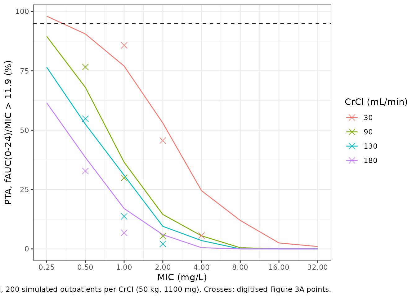
ICU parameter set
# Figure dose response: 1100 mg / 825 mg = 1.33, so for any linear model the
# 50 kg / 1100 mg crossings sit 1.33-fold above the 40 kg / 825 mg crossings
# (weight enters only the volumes, which do not change AUC).
dose_shift <- mic50 |>
  dplyr::filter(panel %in% c("40 kg, 825 mg", "50 kg, 1100 mg")) |>
  dplyr::select(group, panel, crcl, mic50_fig) |>
  tidyr::pivot_wider(names_from = panel, values_from = mic50_fig) |>
  dplyr::mutate(ratio = `50 kg, 1100 mg` / `40 kg, 825 mg`)

icu90 <- dplyr::filter(mic50, group == "ICU", panel == "40 kg, 825 mg", crcl == 90)
icu_auc_model <- 0.80 * 825 / (1.2 * 90 / 101)
icu_auc_fig <- icu90$mic50_fig * 11.9 / 0.88

# Single 825 mg dose from zero, typical ICU patient at the Table 1 medians.
icu_sd <- rxode2::rxSolve(
  mod_typ,
  rxode2::et(amt = 825, cmt = "depot") |> rxode2::et(seq(0, 24, by = 0.05)),
  params = c(DIS_CRITILL = 1, CRCL = 92.3, WT = 51.2, OCC = 1),
  returnType = "data.frame"
)
#> ℹ omega/sigma items treated as zero: 'etalcl_icu', 'etalvc_icu', 'etalka_occ1_icu', 'etalka_occ2_icu', 'etalfdepot_icu', 'etalq_icu', 'etalvp_icu', 'etalcl_outpt', 'etalvc_outpt', 'etalka_occ1_outpt', 'etalka_occ2_outpt', 'etalfdepot_outpt', 'etalq_outpt', 'etalvp_outpt'
icu_cmax_sd <- max(icu_sd$Cc)

# Terminal half-life of the typical ICU patient (CRCL 101, WT 56).
k10 <- 1.2 / 64.8; k12 <- 7.3 / 64.8; k21 <- 7.3 / 348.6
lambda_z <- ((k10 + k12 + k21) - sqrt((k10 + k12 + k21)^2 - 4 * k10 * k21)) / 2
icu_thalf_days <- log(2) / lambda_z / 24

stopifnot(
  abs(stats::median(dose_shift$ratio[dose_shift$group == "Outpatients"]) - 1.33) < 0.1,
  all(dose_shift$ratio[dose_shift$group == "ICU"] < 1.2),
  icu_auc_model > 550, icu_auc_model < 700,
  icu_auc_fig > 15, icu_auc_fig < 30,
  icu_cmax_sd > 6, icu_cmax_sd < 8,
  icu_thalf_days > 8, icu_thalf_days < 12
)
knitr::kable(
  dose_shift |>
    dplyr::rename("Group" = group, "CrCl (mL/min)" = crcl,
                  "1100 / 825 mg crossing ratio (figure)" = ratio),
  digits = 2,
  caption = "Dose response of the published 50% crossings; a linear model gives 1.33."
)| Group | CrCl (mL/min) | 40 kg, 825 mg | 50 kg, 1100 mg | 1100 / 825 mg crossing ratio (figure) |
|---|---|---|---|---|
| ICU | 30 | 4.14 | 3.79 | 0.91 |
| ICU | 90 | 1.79 | 1.88 | 1.05 |
| ICU | 130 | 1.34 | 1.38 | 1.03 |
| ICU | 180 | 0.95 | 1.00 | 1.05 |
| Outpatients | 30 | 1.43 | 1.77 | 1.24 |
| Outpatients | 90 | 0.57 | 0.76 | 1.34 |
| Outpatients | 130 | 0.40 | 0.55 | 1.39 |
| Outpatients | 180 | 0.30 | 0.40 | 1.33 |
The ICU arm does not reproduce the paper. The steady-state ICU
AUC(0-24) implied by Table 3
(0.80 * 825 / (1.2 * CRCL / 101), 617 mg.h/L at 90 mL/min)
is more than 10 times the ICU value implied by Figure 2A (24.3 mg.h/L at
90 mL/min, 40 kg, 825 mg). It is also far above the observed ICU
AUC(0-24) in Table 2 (median 19.61 mg.h/L). With the Table
3 ICU central volume and bioavailability, even a single 825 mg dose from
zero peaks at 7.1 mg/L, three times the observed ICU median
Cmax of 2.33 mg/L. The Figure 2A curves also barely move
between 825 mg and 1100 mg, which no linear model can reproduce, while
the outpatient curves in Figure 3A shift by the expected 1.33-fold. The
published ICU clearance of 1.2 L/h gives a terminal half-life of 11.1
days, and it is also the value the abstract’s “93% lower” is computed
from.
Two things may explain part of the gap. First, the fit used each subject’s measured pre-dose concentration as the initial condition of each 24-hour sampling window, so ICU clearance was informed only by distribution-dominated 24-hour profiles. Second, the NPAG means are not a typical subject. Neither can close a 30-fold gap. The ICU parameters are shipped exactly as printed. They should not be used to predict ICU exposure at steady state; this vignette documents the gap and does not correct it.
Virtual cohort and simulation
The simulated cohort reproduces the sampling design. Each subject takes the weight-banded FDC dose once daily for 10 days before sampling (the median time on treatment, Results 2.1), and the sampled interval is the 11th dose on the paper’s sampling grid. Weight and creatinine clearance are drawn from a piecewise-linear distribution that reproduces the Table 1 median and interquartile range exactly; the outer bounds (not reported) are set by the maintainers. A log-normal fitted to the IQR is not used because the outpatient creatinine-clearance IQR (26.5-157.9 around a median of 113.88 mL/min) is strongly skewed. The cohorts are 100 per group.
rxode2::rxSetSeed(1559)
set.seed(1559) # covariate draws use base R's generator
n_per_group <- 100

# Inverse CDF through (min, Q1, median, Q3, max): reproduces the median and IQR.
draw_iqr <- function(n, lo, q1, median, q3, hi) {
  stats::approx(c(0, 0.25, 0.5, 0.75, 1), c(lo, q1, median, q3, hi), xout = stats::runif(n))$y
}
fdc_dose <- function(wt) ifelse(wt <= 35, 550, ifelse(wt <= 50, 825, 1100))

subj <- dplyr::bind_rows(
  tibble::tibble(
    treatment = "ICU", DIS_CRITILL = 1,
    WT = draw_iqr(n_per_group, 36, 46.2, 51.2, 58.6, 80),
    CRCL = draw_iqr(n_per_group, 10, 36.0, 92.3, 129.1, 200)
  ),
  tibble::tibble(
    treatment = "Outpatients", DIS_CRITILL = 0,
    WT = draw_iqr(n_per_group, 40, 53.2, 58.35, 67, 90),
    CRCL = draw_iqr(n_per_group, 10, 26.5, 113.88, 157.9, 220)
  )
) |>
  dplyr::mutate(id = dplyr::row_number(), OCC = 1, dose = fdc_dose(WT))

t_sample <- 240 + c(0, 0.5, 1, 2, 4, 6, 8, 12, 24)
events <- dplyr::bind_rows(
  subj |> tidyr::crossing(time = seq(0, 240, by = 24)) |>
    dplyr::mutate(amt = dose, evid = 1L, cmt = "depot"),
  subj |> tidyr::crossing(time = t_sample) |>
    dplyr::mutate(amt = NA_real_, evid = 0L, cmt = "central")
) |>
  dplyr::arrange(id, time, dplyr::desc(evid))
stopifnot(!anyDuplicated(events[, c("id", "time", "evid")]))

sim <- rxode2::rxSolve(mod, events, returnType = "data.frame",
                       keep = c("treatment", "dose", "WT", "CRCL"))
# The same cohort with random effects zeroed separates the covariate and the
# IIV contributions in the NCA comparison below.
sim_typ <- rxode2::rxSolve(mod_typ, events, returnType = "data.frame",
                           keep = c("treatment", "dose", "WT", "CRCL"))
#> ℹ omega/sigma items treated as zero: 'etalcl_icu', 'etalvc_icu', 'etalka_occ1_icu', 'etalka_occ2_icu', 'etalfdepot_icu', 'etalq_icu', 'etalvp_icu', 'etalcl_outpt', 'etalvc_outpt', 'etalka_occ1_outpt', 'etalka_occ2_outpt', 'etalfdepot_outpt', 'etalq_outpt', 'etalvp_outpt'
#> Warning: multi-subject simulation without without 'omega'
stopifnot(nrow(sim) == 2L * n_per_group * length(t_sample), !anyNA(sim$Cc), !anyNA(sim_typ$Cc))
sim |>
  dplyr::mutate(tad = time - 240) |>
  dplyr::group_by(treatment, tad) |>
  dplyr::summarise(
    median = stats::median(Cc),
    lo = stats::quantile(Cc, 0.1),
    hi = stats::quantile(Cc, 0.9),
    .groups = "drop"
  ) |>
  ggplot(aes(tad, median, colour = treatment, fill = treatment)) +
  geom_ribbon(aes(ymin = lo, ymax = hi), alpha = 0.2, colour = NA) +
  geom_line() +
  geom_point() +
  scale_y_log10() +
  labs(x = "Time after the 11th daily dose (h)", y = "Ethambutol (mg/L)",
       caption = "Median and 10th-90th percentiles of 100 simulated patients per group.") +
  theme_bw()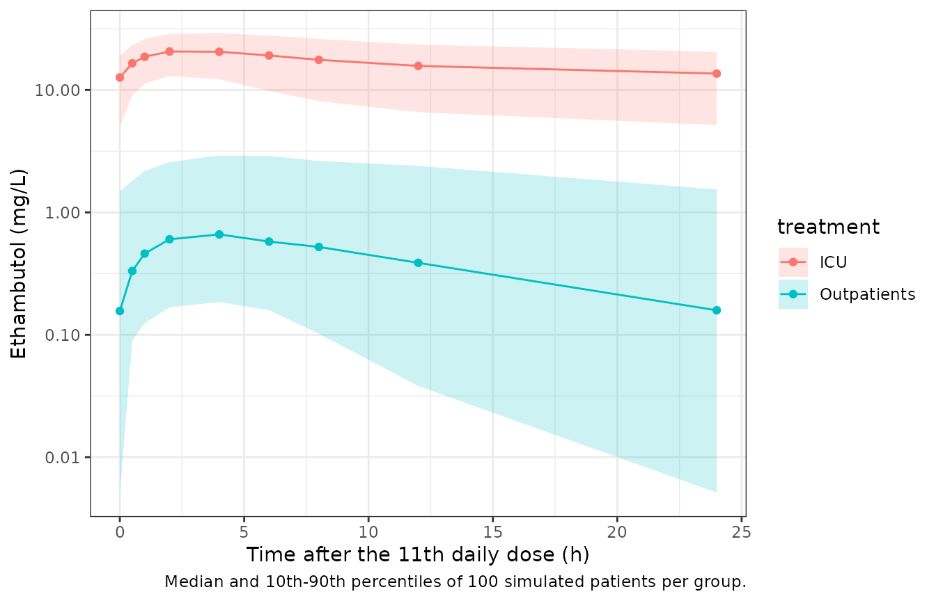
PKNCA validation
doses <- events |>
  dplyr::filter(evid == 1L) |>
  dplyr::select(id, time, amt, treatment)
nca_intervals <- data.frame(start = 240, end = 264, cmax = TRUE, tmax = TRUE, auclast = TRUE)

run_nca <- function(sim_df) {
  conc <- sim_df |>
    dplyr::filter(!is.na(Cc)) |>
    dplyr::select(id, time, Cc, treatment)
  res <- PKNCA::pk.nca(PKNCA::PKNCAdata(
    PKNCA::PKNCAconc(conc, Cc ~ time | treatment + id),
    PKNCA::PKNCAdose(doses, amt ~ time | treatment + id),
    intervals = nca_intervals
  ))
  as.data.frame(res$result)
}
nca_df <- run_nca(sim)
nca_typ_df <- run_nca(sim_typ)
stopifnot(
  nrow(nca_df) == 3L * 2L * n_per_group, !anyNA(nca_df$PPORRES),
  nrow(nca_typ_df) == 3L * 2L * n_per_group, !anyNA(nca_typ_df$PPORRES)
)
Comparison against published NCA
Table 2 reports the observed median Cmax,
AUC(0-24) and Tmax in each group. The
simulated side is summarised as the median over the virtual cohort.
published <- tibble::tribble(
  ~treatment,     ~cmax, ~auclast, ~tmax,
  "ICU",           2.33,   19.61,   2.0,
  "Outpatients",   1.11,    5.52,   2.6
)
simulated <- nca_df |>
  dplyr::group_by(treatment, PPTESTCD) |>
  dplyr::summarise(value = stats::median(PPORRES), .groups = "drop") |>
  tidyr::pivot_wider(names_from = PPTESTCD, values_from = value)

cmp <- nlmixr2lib::ncaComparisonTable(
  simulated = simulated,
  reference = published,
  by = "treatment",
  units = c(cmax = "mg/L", auclast = "mg*h/L", tmax = "h"),
  tolerance_pct = 20
)
knitr::kable(cmp, digits = 2, caption = paste(
  "Simulated (median of 100 per group, 11th daily dose) vs. observed medians in",
  "Table 2 of Beraldi-Magalhaes 2021. * differs by more than 20%."
))| NCA parameter | treatment | Reference | Simulated | % diff |
|---|---|---|---|---|
| Cmax (mg/L) | ICU | 2.33 | 20.8 | +793.9%* |
| Cmax (mg/L) | Outpatients | 1.11 | 0.668 | -39.8%* |
| Tmax (h) | ICU | 2 | 2 | +0.0% |
| Tmax (h) | Outpatients | 2.6 | 4 | +53.8%* |
| AUClast (mg*h/L) | ICU | 19.6 | 398 | +1930.8%* |
| AUClast (mg*h/L) | Outpatients | 5.52 | 9.9 | +79.3%* |
simulated_typ <- nca_typ_df |>
  dplyr::group_by(treatment, PPTESTCD) |>
  dplyr::summarise(value = stats::median(PPORRES), .groups = "drop") |>
  tidyr::pivot_wider(names_from = PPTESTCD, values_from = value)

sim_out <- dplyr::filter(simulated, treatment == "Outpatients")
typ_out <- dplyr::filter(simulated_typ, treatment == "Outpatients")
sim_icu <- dplyr::filter(simulated, treatment == "ICU")
stopifnot(
  # Outpatients, random effects zeroed: the covariate distribution alone puts
  # the cohort median AUC(0-24) within 50% of the observed median. The
  # covariate draw is fixed by set.seed(), so this is deterministic.
  abs(typ_out$auclast / 5.52 - 1) < 0.5,
  # Adding the independent log-normal IIV raises the cohort median (see text).
  sim_out$auclast > typ_out$auclast,
  # ICU: the published parameters over-predict the observed exposure > 5-fold.
  sim_icu$auclast / 19.61 > 5,
  sim_icu$cmax / 2.33 > 3
)
Outpatients. With random effects zeroed, the
cohort’s median AUC(0-24) is 7.79 mg.h/L against the
observed 5.52 mg.h/L, consistent with the Figure 3A crossings above.
Adding the Table 3 variability raises the median to 9.9 mg.h/L. The
independent log-normal F and CL spread
F / CL more widely than the published fit, and combined
with the right-skewed creatinine-clearance distribution, this lifts the
cohort median. The simulated median Cmax is 60% of the
observed median and Tmax differs from the observed value.
That is expected for NPAG marginal means: feeding the mean
ka, Vc and Q into the structural
model does not give the mean of the individual peaks. For that reason
only AUC-based quantities are gated for this arm.
ICU. Every exposure metric is over-predicted several-fold, as explained in the ICU parameter set section. After 10 days the simulated ICU patients have accumulated drug that the observed ICU patients did not have.
Assumptions and deviations
-
Group-specific parameters. The paper estimated
every structural parameter separately for ICU patients and outpatients
in one Pmetrics model. They are encoded as
_icu/_outptstratum-suffixed parameters with their own IIV, selected byDIS_CRITILL. In this cohort ICU admission also means mechanical ventilation and a crushed tablet given by nasogastric tube, so the indicator carries route and formulation as well as critical illness. -
NPAG means as typical values. Table 3 means are
used as typical values, and each %CV is carried as a log-normal variance
log(CV^2 + 1). The NPAG distribution is non-parametric and, for three outpatient parameters, left-skewed (mean below median), so this is an approximation. No covariances are reported and none are encoded. The Figure 3A curves suggestFandCLwere strongly positively correlated, so the model’s variability inF / CLis too wide. With a log-normalF, a small fraction of subjects hasF > 1(0.44% of outpatients and 0.23% of ICU patients). -
Creatinine clearance form. “Normalized to 101
mL/min on clearance” is encoded as the ratio
CRCL / 101. The figures suggest a sub-linear relationship (exponent near 0.8), which the paper does not report. CRCL is the measured 8-hour creatinine clearance in mL/min (Table 1), not BSA-normalised, although Methods 4.6 labels the simulated values mL/min/1.73 m^2. -
Weight exponent. “An allometric scaler (raised to
the 25th power)” on both volumes is read as
(WT / 56)^0.25, fixed. A literal exponent of 25 is not plausible. Because weight only affects the volumes, this choice does not change any AUC above. -
Absorption by occasion.
katakes the first-occasion value whenOCC = 1and the second-occasion value forOCC >= 2. In the study the occasions were the sampled doses on enrolment days 1 and 3. For simulations of routine therapy,OCC = 1throughout is a reasonable default; the two values differ by less than 12%. - Initial conditions. The fit used each subject’s pre-dose concentration as the initial condition of each sampling window. That is a data-fitting device and is not part of the packaged model, which starts from zero drug.
-
Residual error. Not reported (only the form of the
Pmetrics error model is described), so
propSdandaddSdarefixed(0)andCcis an individual prediction without observation noise. - ICU arm. Shipped as printed, but it does not reproduce the paper’s own observed ICU exposures (Table 2) or ICU target-attainment simulations (Figure 2A). See the ICU parameter set section.
- Ka contrasts. The Discussion reports ICU absorption as 192% and 205% higher for the first and second dose. Table 3 gives 206% and 192%, the same numbers in the opposite order. Table 3 is used.
- Figure digitisation. The Figure 2A and 3A points were digitised by the maintainers from the marker positions in the published panels. The table of fractional target attainment (Table 4) is not reproduced: its layout is corrupted in the source (duplicated columns), and it needs the EUCAST MIC distribution, which the paper does not tabulate.