Baricitinib (Decker 2026) • nlmixr2lib

Model and source

Citation: Decker RL, Ernest CS II, Radtke DB, Prakash A, Zhang X. A population pharmacokinetic and exposure-response analysis for baricitinib in pediatric patients with atopic dermatitis. Clin Pharmacokinet 2026;65(1):119-131. doi:10.1007/s40262-025-01563-8.
Description: Two-compartment population PK model with zero-order absorption, an absorption lag, and fixed allometric scaling for oral baricitinib in 393 pediatric patients aged 2 to <18 years with moderate-to-severe atopic dermatitis (BREEZE-AD-PEDS, NCT03952559). Apparent total clearance is partitioned semi-mechanistically into an eGFR-dependent apparent renal arm (CLr/F) and an eGFR-independent apparent non-renal arm (CLnr/F). Baseline body weight enters through allometric exponents fixed at 0.75 on all clearance terms (CLr/F, CLnr/F, Q) and at 1 on both volumes (V1/F, V2/F), referenced to 74 kg. The structure was carried unchanged from the adult atopic-dermatitis baricitinib population PK model; no further covariate met the stepwise-covariate-modeling inclusion criteria, so the base model is the final model.
Article: https://doi.org/10.1007/s40262-025-01563-8

Baricitinib is an oral Janus-kinase inhibitor selective for JAK1 and JAK2. Decker and colleagues took the population PK model previously developed in adult patients with atopic dermatitis (AD), added allometric scaling on body weight with the exponents fixed at the canonical 0.75 and 1, and re-estimated it against data from the phase 3 BREEZE-AD-PEDS trial in patients aged 2 to <18 years with moderate-to-severe AD. The purpose of the analysis was to convert the trial’s age-based dosing into a weight-based posology reproducing the adult 4 mg once-daily exposure. The resulting recommendation - 2 mg once daily for 10 to <30 kg and 4 mg once daily for at least 30 kg - is the authorised European pediatric AD posology.

The structural model is a two-compartment model with zero-order absorption over a duration D1 after a lag LAG, dosed directly into the central compartment. Apparent total clearance is partitioned semi-mechanistically:

CLr/F, an apparent renal arm scaled by the patient’s baseline estimated glomerular filtration rate (eGFR, bedside Schwartz), representing renal filtration and secretion - the primary elimination route for baricitinib;
CLnr/F, an apparent eGFR-independent arm, largely hepatic metabolism.

Body weight enters both arms and Q with an exponent fixed at 0.75, and both volumes with an exponent fixed at 1, referenced to 74 kg. Age, sex and race were screened by stepwise covariate modeling and none met the inclusion criteria, so the base model is the final model.

This paper is a sibling of Decker_2024_baricitinib, which applies the same model structure to pediatric juvenile idiopathic arthritis. The two share a structure but not a single parameter value; both are packaged separately.

The paper’s exposure-response analysis (Figures 4 and 5) is a descriptive summary of vIGA-AD 0/1 response rates by steady-state average-concentration quartile. It reports no fitted E-R parameters - no slope, no EC50, no logistic intercept - so there is no E-R model to encode. Only the population PK model is packaged here.

Population

The population PK dataset held 2035 baricitinib concentrations from 393 participants aged 2 to <18 years with moderate-to-severe AD. One participant was later excluded from the reported demographics because of an erroneous screening weight, so Table S1 summarises 392. Mean age was 12.0 years (range 2.00-17.9) and 72% of patients were in the 10 to <18 year band. Mean body weight was 46.6 kg (range 12.0-104 kg), with 78% of patients weighing at least 30 kg. 197 of 392 patients (50%) were female and 287 (73%) were White; 76 (19%) were Asian. Mean baseline eGFR, computed with the bedside Schwartz equation, was 109 mL/min/1.73 m^2 (range 54.3-196); screening eGFR had to exceed 60 mL/min/1.73 m^2.

Dosing during the trial was age-based. The open-label PK lead-in used the “high” dose for each band (4 mg once daily for 10 to <18 years, 2 mg once daily for 2 to <10 years); the 16-week double-blind period randomised 1:1:1:1 to placebo or a low, medium or high dose, which in absolute terms was 1, 2 or 4 mg for ages 10 to <18 years and 0.5, 1 or 2 mg for ages 2 to <10 years. Lead-in samples were collected as dried whole blood on a Mitra VAMS microsampling device and converted to plasma equivalents using a study-specific blood/plasma ratio of 1.32 (Figure S7, 15 concordance pairs), then pooled with the plasma samples.

The same information is available programmatically via readModelDb("Decker_2026_baricitinib")()$population.

Source trace

Every ini() entry in inst/modeldb/specificDrugs/Decker_2026_baricitinib.R carries an in-file comment naming its origin. They are collected here for review. Structural values come from Table 1 (“Pharmacokinetic and covariate parameters in final population model”), Population mean (%SEE) column. The between-subject variances come from ESM Table S2 (“Correlation Matrix for the Final Model”), for the reason set out immediately below the table.

Equation / parameter	Value	Source location
`ld1` (D1)	0.263 h	Table 1, D1 (%SEE 8.86)
`boxcox_d1`	0.311	Table 1, “Box-Cox transformation parameter for D1” (%SEE 6.85)
`ltlag` (LAG)	0.144 h	Table 1, LAG (%SEE 1.73)
`lcl_nonren` (CLnr/F)	2.76 L/h	Table 1, CLnr/F (%SEE 15.4)
`lcl_renal` (CLr/F)	7.9 L/h	Table 1, CLr/F (%SEE 12.1)
`lvc` (V1/F)	119 L	Table 1, V1/F (%SEE 4.12)
`lq` (Q)	2.4 L/h	Table 1, Q (%SEE 9.17)
`lvp` (V2/F)	46.8 L	Table 1, V2/F (%SEE 14.7)
`e_wt_cl_q`	0.75 (fixed)	Table 1, “Allometric scaling CL” = 0.75 (FIX); footnotes b, d
`e_wt_vc_vp`	1 (fixed)	Table 1, “Allometric scaling V” = 1 (FIX); footnotes c, e
`e_dcrcl_cl_renal`	0.00778	Table 1, “Covariate for change in eGFR on CLr/F” (%SEE 42.5)
`etald1` variance	1.30	ESM Table S2, D1 Estimate (RSE 13.9)
`etalcl_nonren` variance	0.313	ESM Table S2, CLnr Estimate (RSE 4.54)
`etalcl_renal` variance	0.358	ESM Table S2, CLr Estimate (RSE 16.5)
`etalvc` variance	0.0161	ESM Table S2, V1 Estimate (RSE 19.9)
`etalvp` variance	0.848	ESM Table S2, V2 Estimate (RSE 44.3)
`etalq` variance	0.0225 (fixed)	ESM Table S2, Q Estimate (fixed)
cov(CLnr/F, CLr/F)	0.303	Table 1, “Covariance for CLnr/F and CLr/F”; footnote g
cov(CLr/F, V1/F)	-0.0265	Table 1, “Covariance for CLr/F and V1/F”; footnote g
cov(CLnr/F, V1/F)	0 (fixed)	ESM Table S2 gives corr(CLnr, V1) = 0.00 explicitly
`propSd`	0.427	Table 1, “Proportional error”; footnote h: standard deviation
Total clearance `cl <- cl_renal + cl_nonren`	n/a	Table 1 footnote b
Allometric scaling `(WT/74)^0.75` on CLr/F, CLnr/F, Q	n/a	Table 1 footnotes b, d
Allometric scaling `(WT/74)^1.00` on V1/F, V2/F	n/a	Table 1 footnotes c, e
Renal-arm eGFR scaling `(CRCL_BASE/93) + 0.00778*(CRCL - CRCL_BASE)`	n/a	Table 1 footnote f
Two-compartment structure; zero-order input into `central` with duration D1 and lag LAG; no depot state	n/a	Methods, “PK Model Development”; Figure S1 legend (compartments C and Cp only)

Reconciling the two reports of the between-subject variances

The paper reports the BSV twice, in two different parameterisations, and they do not agree. Table 1 gives a %CV column with footnote a defining %CV = (sqrt(exp(OMEGA)-1))*100. ESM Table S2 gives the OMEGA variances directly in its Estimate column, with a matrix whose diagonal holds the corresponding standard deviations and whose off-diagonal holds correlations.

Three checks establish which report to encode.

# ESM Table S2, "Estimate" column (the OMEGA variances) and the diagonal of the
# accompanying matrix (which Table S2 prints as standard deviations).
s2 <- tibble::tribble(
  ~param, ~variance_S2, ~sd_S2_printed, ~rse_S2, ~cv_pct_T1,
  "D1",         1.30,          1.14,      13.9,       164,
  "CLnr/F",     0.313,         0.559,      4.54,       58.4,
  "CLr/F",      0.358,         0.598,     16.5,        62.3,
  "V1/F",       0.0161,        0.127,     19.9,        12.7,
  "V2/F",       0.848,         0.921,     44.3,       117,
  "Q",          0.0225,        0.150,      NA,         15.1
) |>
  mutate(
    `sqrt(variance)`      = sqrt(variance_S2),
    `%CV implied by S2`   = sqrt(exp(variance_S2) - 1) * 100,
    `%CV round-trips?`    = ifelse(abs(`%CV implied by S2` - cv_pct_T1) < 1.5, "yes", "NO")
  )

s2 |>
  dplyr::rename(
    "Parameter"                 = param,
    "Variance (Table S2)"       = variance_S2,
    "SD printed (Table S2)"     = sd_S2_printed,
    "RSE% (Table S2)"           = rse_S2,
    "%CV (Table 1)"             = cv_pct_T1
  ) |>
  knitr::kable(
    digits  = c(0, 4, 3, 2, 1, 4, 1, 0),
    caption = paste(
      "Check 1: Table S2's variances reproduce its own printed SD diagonal for",
      "all six terms, but Table 1's %CV column round-trips for only four."
    )
  )

Check 1: Table S2’s variances reproduce its own printed SD diagonal for all six terms, but Table 1’s %CV column round-trips for only four.
Parameter	Variance (Table S2)	SD printed (Table S2)	RSE% (Table S2)	%CV (Table 1)	sqrt(variance)	%CV implied by S2	%CV round-trips?
D1	1.3000	1.140	13.90	164.0	1.1402	163.4	yes
CLnr/F	0.3130	0.559	4.54	58.4	0.5595	60.6	NO
CLr/F	0.3580	0.598	16.50	62.3	0.5983	65.6	NO
V1/F	0.0161	0.127	19.90	12.7	0.1269	12.7	yes
V2/F	0.8480	0.921	44.30	117.0	0.9209	115.5	yes
Q	0.0225	0.150	NA	15.1	0.1500	15.1	yes

Check 1 - the square roots of Table S2’s variances reproduce Table S2’s own printed standard-deviation diagonal exactly for all six terms. Table 1’s %CV column, back-transformed through its footnote a, reproduces Table S2 for D1, V1/F, Q and V2/F but not for CLnr/F (58.4% implies a variance of 0.293, versus 0.313) or CLr/F (62.3% implies 0.328, versus 0.358). Table S2’s RSE% column matches Table 1’s %SEE column for every one of the six terms, so the two tables unambiguously describe the same fit.

Check 2 - Table S2’s off-diagonal correlations, combined with its own standard deviations, reproduce Table 1’s two reported covariances.

sd_clnr <- sqrt(0.313); sd_clr <- sqrt(0.358); sd_v1 <- sqrt(0.0161)

tibble::tibble(
  Pair            = c("CLnr/F & CLr/F", "CLr/F & V1/F"),
  `corr (Tab S2)` = c(0.904, -0.349),
  `corr x SD x SD` = c(0.904 * sd_clnr * sd_clr, -0.349 * sd_clr * sd_v1),
  `cov reported (Tab 1)` = c(0.303, -0.0265)
) |>
  knitr::kable(
    digits  = 5,
    caption = "Check 2: Table S2's correlations reproduce Table 1's covariances."
  )

Check 2: Table S2’s correlations reproduce Table 1’s covariances.
Pair	corr (Tab S2)	corr x SD x SD	cov reported (Tab 1)
CLnr/F & CLr/F	0.904	0.30261	0.3030
CLr/F & V1/F	-0.349	-0.02650	-0.0265

Check 3 - the decisive one. A covariance matrix must be positive definite. Reconstructing the block from Table 1’s %CV column while keeping Table 1’s own covariances gives an impossible matrix; using Table S2’s variances gives a valid one.

build_block <- function(v_clnr, v_clr, v_v1) {
  matrix(
    c(v_clnr,  0.303,   0,
      0.303,   v_clr,  -0.0265,
      0,      -0.0265,  v_v1),
    nrow = 3, byrow = TRUE,
    dimnames = list(c("CLnr", "CLr", "V1"), c("CLnr", "CLr", "V1"))
  )
}

cv2var <- function(cv) log(cv^2 + 1)

# (a) Table 1 %CV column -> variances, with Table 1 covariances.
blk_t1 <- build_block(cv2var(0.584), cv2var(0.623), cv2var(0.127))
round(eigen(blk_t1)$values, 6)
#> [1]  0.614818  0.029939 -0.007343

# (b) ESM Table S2 variances, with Table 1 covariances. This is what is encoded.
blk_s2 <- build_block(0.313, 0.358, 0.0161)
round(eigen(blk_s2)$values, 6)
#> [1] 0.639939 0.043333 0.003828

# (a) has a negative eigenvalue and cannot be sampled from; (b) is valid.
stopifnot(min(eigen(blk_t1)$values) < 0)
stopifnot(min(eigen(blk_s2)$values) > 0)

# Implied correlations of the encoded block: the two clearance arms are very
# strongly but not perfectly correlated, matching Table S2's printed 0.904.
round(stats::cov2cor(blk_s2), 3)
#>       CLnr    CLr     V1
#> CLnr 1.000  0.905  0.000
#> CLr  0.905  1.000 -0.349
#> V1   0.000 -0.349  1.000

The model therefore encodes the ESM Table S2 variances together with Table 1’s covariances. The alternative is not merely less well supported, it is arithmetically impossible.

Independent anchors

Two anchors confirm the structural transcription without any simulation. At the reference weight of 74 kg and the reference eGFR of 93 mL/min/1.73 m^2 the model gives CLr/F + CLnr/F = 7.9 + 2.76 = 10.66 L/h, matching the paper’s statement that “the total clearance estimate (for a weight of 74 kg) is 10.7 L/h”. The reference eGFR of 93 is therefore load-bearing: it is the median eGFR of the upstream adult analysis, not a statistic of this pediatric cohort (whose mean baseline eGFR is 109).

c(`CL/F at 74 kg, eGFR 93 (L/h)` = 7.9 + 2.76, `paper text` = 10.7)
#> CL/F at 74 kg, eGFR 93 (L/h)                   paper text 
#>                        10.66                        10.70

Are the Table 2 exposure columns internally consistent?

Table 2 reports post-hoc parameter and exposure estimates by age group, by weight group and by dose. Before using it as a validation target it is worth checking a property the model must satisfy regardless of any parameter value: at steady state under linear PK, AUC(tau,ss) must equal Dose / (CL/F).

t2 <- tibble::tribble(
  ~group,          ~dose_mg, ~cl,   ~auc, ~cmax, ~n,
  "2 to <6 y",          0.5,  5.29,  94.3, 18.9,   9,
  "2 to <6 y",            1,  4.98, 200,   35.1,   8,
  "2 to <6 y",            2,  6.69, 298,   64.8,  15,
  "6 to <10 y",         0.5,  6.67,  74.8, 11.6,  24,
  "6 to <10 y",           1,  6.42, 155,   23.1,  26,
  "6 to <10 y",           2,  7.14, 279,   45.7,  29,
  "10 to <18 y",          1,  9.16, 109,   13.2,  87,
  "10 to <18 y",          2,  8.98, 222,   27.8,  86,
  "10 to <18 y",          4, 10.40, 383,   50.7, 108,
  "< 30 kg",              2,  6.70, 298,   57.1,  35,
  ">= 30 kg",             4, 10.40, 383,   50.3, 106,
  "Adult AD (reference)", 4, 10.50, 380,   45.0, 819
) |>
  mutate(
    `AUC implied by Dose/CL` = dose_mg / cl * 1000,
    `% difference`           = 100 * (auc - `AUC implied by Dose/CL`) /
                                 `AUC implied by Dose/CL`
  )

t2 |>
  dplyr::rename(
    "Group"              = group,
    "N"                  = n,
    "Dose (mg)"          = dose_mg,
    "CL/F (L/h)"         = cl,
    "AUCtau,ss reported" = auc,
    "Cmax,ss reported"   = cmax
  ) |>
  knitr::kable(
    digits  = 1,
    caption = paste(
      "Internal consistency of Decker 2026 Table 2. Under linear steady-state",
      "PK, AUC(tau,ss) must equal Dose/(CL/F)."
    )
  )

Internal consistency of Decker 2026 Table 2. Under linear steady-state PK, AUC(tau,ss) must equal Dose/(CL/F).
Group	Dose (mg)	CL/F (L/h)	AUCtau,ss reported	Cmax,ss reported	N	AUC implied by Dose/CL	% difference
2 to <6 y	0.5	5.3	94.3	18.9	9	94.5	-0.2
2 to <6 y	1.0	5.0	200.0	35.1	8	200.8	-0.4
2 to <6 y	2.0	6.7	298.0	64.8	15	299.0	-0.3
6 to <10 y	0.5	6.7	74.8	11.6	24	75.0	-0.2
6 to <10 y	1.0	6.4	155.0	23.1	26	155.8	-0.5
6 to <10 y	2.0	7.1	279.0	45.7	29	280.1	-0.4
10 to <18 y	1.0	9.2	109.0	13.2	87	109.2	-0.2
10 to <18 y	2.0	9.0	222.0	27.8	86	222.7	-0.3
10 to <18 y	4.0	10.4	383.0	50.7	108	384.6	-0.4
< 30 kg	2.0	6.7	298.0	57.1	35	298.5	-0.2
>= 30 kg	4.0	10.4	383.0	50.3	106	384.6	-0.4
Adult AD (reference)	4.0	10.5	380.0	45.0	819	381.0	-0.2


# Every row must reconcile to within 1%; assert rather than eyeball.
stopifnot(max(abs(t2$`% difference`)) < 1)

Every one of the twelve columns reconciles to better than 1%. This is a stronger starting position than the sibling JIA analysis, where the age-based dosing left one weight-group column inconsistent with its own printed dose. Here the weight groups are explicitly restricted (Table 2 footnote d) to patients who received the dose that the weight-based posology would assign - 2 mg below 30 kg and 4 mg at or above 30 kg - so both weight-group columns are valid targets.

Virtual cohort

Original individual data are not publicly available. Each arm below reproduces one Table 2 column, with body weight drawn to match that column’s mean and range and baseline eGFR drawn to match the corresponding stratum of Table S1, at the dose the column reports.

Arm	Table 2 N	Dose	Weight, mean (range)	Baseline eGFR, mean (range)
2 to <6 y	15	2 mg QD	17.4 kg (12.0-25.0)	124 (73.2-164)
6 to <10 y	29	2 mg QD	28.5 kg (17.0-59.3)	127 (92.6-195)
10 to <18 y	108	4 mg QD	55.0 kg (24.4-104)	103 (54.3-196)
< 30 kg	35	2 mg QD	21.5 kg (13.4-29.7)	125 (73.2-195)
>= 30 kg	106	4 mg QD	56.9 kg (31.0-104)	105 (54.3-196)

Weight means and ranges for the age-group arms come from Table 2’s “Weight (kg)” row, which coincides with Table S1’s age-group weights. The two weight-group arms use Table 2’s weight statistics (21.5 and 56.9 kg) rather than Table S1’s (21.9 and 53.7 kg), because Table 2 footnote d restricts those columns to the correctly-dosed subset that produced the exposure targets. eGFR statistics come from Table S1 throughout.

set.seed(20260220)

# Rejection-sample a truncated normal matched to a reported mean and range.
rtrunc_norm <- function(n, mean, lo, hi) {
  if (isTRUE(all.equal(lo, hi))) return(rep(mean, n))
  sd  <- (hi - lo) / 4
  out <- numeric(0)
  while (length(out) < n) {
    x   <- stats::rnorm(4 * n, mean = mean, sd = sd)
    out <- c(out, x[x >= lo & x <= hi])
  }
  out[seq_len(n)]
}

# Steady-state design: QD dosing for 8 days, then a densely sampled final
# dosing interval. The terminal half-life reaches ~17 h in the largest patients,
# so 8 daily doses leave the trough within 0.1% of steady state; the assertion
# after the simulation checks this rather than assuming it.
tau      <- 24
n_doses  <- 8L
ss_start <- (n_doses - 1L) * tau          # 168 h -- time of the final dose
obs_grid <- sort(unique(c(
  seq(ss_start,       ss_start + 2,   by = 0.10),   # capture the sharp peak
  seq(ss_start + 2.5, ss_start + 12,  by = 0.50),
  seq(ss_start + 13,  ss_start + tau, by = 1.00)
)))

# Build one arm. `id_offset` keeps IDs disjoint across bind_rows()-ed arms;
# duplicate IDs are silently merged by rxSolve into a single wrong subject.
make_arm <- function(n, amt_mg, wt_mean, wt_lo, wt_hi,
                     egfr_mean, egfr_lo, egfr_hi, treatment, id_offset = 0L) {
  subj <- tibble(
    id        = id_offset + seq_len(n),
    WT        = rtrunc_norm(n, wt_mean, wt_lo, wt_hi),
    CRCL_BASE = rtrunc_norm(n, egfr_mean, egfr_lo, egfr_hi),
    treatment = treatment
  ) |>
    # The paper reports no on-treatment eGFR trajectory, so the time-varying
    # arm is switched off by setting CRCL == CRCL_BASE (delta-eGFR = 0).
    mutate(CRCL = CRCL_BASE)

  doses <- subj |>
    tidyr::crossing(time = seq(0, by = tau, length.out = n_doses)) |>
    mutate(
      amt  = amt_mg,
      evid = 1L,
      cmt  = "central",
      # rate = -2 tells rxode2 the infusion DURATION is modeled -- here by
      # dur(central) <- d1 in the model file. Without it the zero-order
      # absorption duration D1 is ignored and the dose becomes a bolus.
      rate = -2
    )

  obs <- subj |>
    tidyr::crossing(time = obs_grid) |>
    mutate(
      amt  = NA_real_,
      evid = 0L,
      # The ODE state name, never the observable name "Cc" -- referencing an
      # algebraic observable as a compartment renumbers the ODE slots.
      cmt  = "central",
      rate = NA_real_
    )

  bind_rows(doses, obs) |> arrange(id, time, desc(evid))
}

arms <- tibble::tribble(
  ~treatment,     ~amt_mg, ~wt_mean, ~wt_lo, ~wt_hi, ~egfr_mean, ~egfr_lo, ~egfr_hi,
  "2 to <6 y",          2,     17.4,   12.0,   25.0,        124,     73.2,      164,
  "6 to <10 y",         2,     28.5,   17.0,   59.3,        127,     92.6,      195,
  "10 to <18 y",        4,     55.0,   24.4,  104.0,        103,     54.3,      196,
  "< 30 kg",            2,     21.5,   13.4,   29.7,        125,     73.2,      195,
  ">= 30 kg",           4,     56.9,   31.0,  104.0,        105,     54.3,      196
) |>
  mutate(id_offset = 1000L * seq_len(dplyr::n()))

n_per_arm <- 150L

events <- do.call(bind_rows, lapply(seq_len(nrow(arms)), function(i) {
  a <- arms[i, ]
  make_arm(n_per_arm, a$amt_mg, a$wt_mean, a$wt_lo, a$wt_hi,
           a$egfr_mean, a$egfr_lo, a$egfr_hi, a$treatment, a$id_offset)
}))

# A genuine duplicate check: anyDuplicated() on the key columns themselves.
stopifnot(anyDuplicated(events[, c("id", "time", "evid")]) == 0L)
c(arms = nrow(arms), subjects = dplyr::n_distinct(events$id), rows = nrow(events))
#>     arms subjects     rows 
#>        5      750    45750

Simulation

mod <- readModelDb("Decker_2026_baricitinib")

sim <- rxode2::rxSolve(
  mod,
  events = events,
  keep   = c("treatment", "WT", "CRCL_BASE")
) |>
  as.data.frame()
#> ℹ parameter labels from comments will be replaced by 'label()'

# rxSolve can silently drop subjects; assert the count survived.
stopifnot(dplyr::n_distinct(sim$id) == dplyr::n_distinct(events$id))
c(subjects_out = dplyr::n_distinct(sim$id), rows_out = nrow(sim))
#> subjects_out     rows_out 
#>          750        39750

The design assumes 8 daily doses reach steady state. Verify it rather than assert it, by comparing the trough at the start of the final interval against the trough 24 h earlier.

troughs <- rxode2::rxSolve(
  mod,
  events = events |> filter(evid == 1L | time %in% c(ss_start - tau, ss_start)),
  keep   = c("treatment")
) |>
  as.data.frame() |>
  filter(time %in% c(ss_start - tau, ss_start)) |>
  group_by(time) |>
  summarise(median_trough = median(Cc), .groups = "drop")

ss_gap <- 100 * diff(troughs$median_trough) / troughs$median_trough[1]
c(troughs$median_trough, `% change in trough over final 24 h` = ss_gap)
#>          
#> 3.447577

# Steady state is reached if the last two troughs agree to better than 1%.
stopifnot(abs(ss_gap) < 1)

Structural check against Table 2

The model’s only structural covariates are body weight and baseline eGFR, so the typical-value parameters evaluated at each group’s mean weight and mean eGFR can be compared directly against the post-hoc geometric means in Table 2. This is deterministic, so between-subject variability is zeroed.

# zeroRe() removes the random effects. omega = NA is passed explicitly because
# rxSolve() otherwise reuses the omega from the previous solve in the session.
mod_typical <- rxode2::zeroRe(mod)
#> ℹ parameter labels from comments will be replaced by 'label()'

typ_events <- do.call(bind_rows, lapply(seq_len(nrow(arms)), function(i) {
  a <- arms[i, ]
  make_arm(1L, a$amt_mg, a$wt_mean, a$wt_mean, a$wt_mean,
           a$egfr_mean, a$egfr_mean, a$egfr_mean, a$treatment, a$id_offset)
}))

sim_typ <- rxode2::rxSolve(
  mod_typical, events = typ_events, omega = NA,
  keep = c("treatment", "WT", "CRCL_BASE")
) |>
  as.data.frame()
#> Warning: multi-subject simulation without without 'omega'

# Terminal (beta) half-life of a two-compartment model from the micro-constants.
terminal_half_life <- function(cl, vc, q, vp) {
  k10  <- cl / vc
  k12  <- q / vc
  k21  <- q / vp
  a    <- k10 + k12 + k21
  beta <- (a - sqrt(a^2 - 4 * k10 * k21)) / 2
  log(2) / beta
}

typ_tbl <- sim_typ |>
  group_by(treatment) |>
  summarise(
    cl_model    = mean(cl),
    # Table 2 footnote f defines V/F as V1/F + V2/F.
    v_model     = mean(vc) + mean(vp),
    thalf_model = terminal_half_life(mean(cl), mean(vc), mean(q), mean(vp)),
    .groups = "drop"
  )

published_t2 <- tibble::tribble(
  ~treatment,    ~cl_pub, ~v_pub, ~thalf_pub,
  "2 to <6 y",      6.69,   38.9,       10.7,
  "6 to <10 y",     7.14,   63.4,       13.2,
  "10 to <18 y",   10.40,  119.0,       16.0,
  "< 30 kg",        6.70,   47.1,       11.7,
  ">= 30 kg",      10.40,  120.0,       16.1
)

typ_tbl |>
  left_join(published_t2, by = "treatment") |>
  mutate(`CL/F % diff` = 100 * (cl_model - cl_pub) / cl_pub,
         `V/F % diff`  = 100 * (v_model - v_pub) / v_pub,
         `t1/2 % diff` = 100 * (thalf_model - thalf_pub) / thalf_pub) |>
  dplyr::rename(
    "Group"              = treatment,
    "CL/F model (L/h)"   = cl_model,
    "CL/F Table 2 (L/h)" = cl_pub,
    "V/F model (L)"      = v_model,
    "V/F Table 2 (L)"    = v_pub,
    "t1/2 model (h)"     = thalf_model,
    "t1/2 Table 2 (h)"   = thalf_pub
  ) |>
  dplyr::relocate(`CL/F % diff`, .after = `CL/F Table 2 (L/h)`) |>
  dplyr::relocate(`V/F % diff`,  .after = `V/F Table 2 (L)`) |>
  dplyr::relocate(`t1/2 % diff`, .after = `t1/2 Table 2 (h)`) |>
  knitr::kable(
    digits  = 1,
    caption = paste(
      "Typical-value structural parameters versus the post-hoc geometric means",
      "of Decker 2026 Table 2."
    )
  )

Typical-value structural parameters versus the post-hoc geometric means of Decker 2026 Table 2.
Group	CL/F model (L/h)	V/F model (L)	t1/2 model (h)	CL/F Table 2 (L/h)	CL/F % diff	V/F Table 2 (L)	V/F % diff	t1/2 Table 2 (h)	t1/2 % diff
10 to <18 y	9.2	123.2	16.9	10.4	-11.4	119.0	3.6	16.0	5.4
2 to <6 y	4.5	39.0	12.1	6.7	-32.9	38.9	0.2	10.7	12.7
6 to <10 y	6.6	63.9	13.6	7.1	-7.2	63.4	0.7	13.2	2.8
< 30 kg	5.3	48.2	12.7	6.7	-21.0	47.1	2.3	11.7	8.5
>= 30 kg	9.6	127.5	16.9	10.4	-7.8	120.0	6.2	16.1	5.1

V/F reproduces Table 2 to within 6% in every arm and to within 1% in the two smallest, which is expected: both volumes scale linearly with weight (exponent fixed at 1), so the typical value at the group mean weight and the geometric mean of the individual estimates nearly coincide. Terminal half-life reproduces to within 13%.

Clearance shows a systematic pattern: the typical value sits below the post-hoc geometric mean, and the gap widens as body weight falls (-7.8% at 56.9 kg, -21% at 21.5 kg, -33% at 17.4 kg). The paper itself supplies the explanation. Its Discussion reports a sensitivity analysis in which the allometric exponents were estimated instead of fixed, returning 0.59 for clearance-related and 0.66 for volume-related parameters. An exponent shallower than 0.75 means clearance falls less steeply as weight decreases, so the fixed-0.75 model necessarily under-predicts clearance in the smallest patients relative to their individual fits. Substituting the paper’s own estimated exponent closes the gap on the two weight-group arms almost exactly, and both land at the same residual:

# Diagnostic ONLY -- the packaged model keeps the published fixed exponent of
# 0.75 (Table 1, FIX). This recomputes the typical CL/F under the exponent the
# paper's own sensitivity analysis estimated (0.59, Discussion) to show that the
# exponent choice, not a transcription error, drives the residual pattern.
cl_typical <- function(wt, egfr, exponent) {
  (7.9 * (egfr / 93) + 2.76) * (wt / 74)^exponent
}

arms |>
  transmute(
    Group                   = treatment,
    `Weight (kg)`           = wt_mean,
    `CL/F Table 2 (L/h)`    = published_t2$cl_pub[match(treatment, published_t2$treatment)],
    `CL/F at exponent 0.75` = cl_typical(wt_mean, egfr_mean, 0.75),
    `CL/F at exponent 0.59` = cl_typical(wt_mean, egfr_mean, 0.59)
  ) |>
  mutate(
    `% diff at 0.75` = 100 * (`CL/F at exponent 0.75` - `CL/F Table 2 (L/h)`) / `CL/F Table 2 (L/h)`,
    `% diff at 0.59` = 100 * (`CL/F at exponent 0.59` - `CL/F Table 2 (L/h)`) / `CL/F Table 2 (L/h)`
  ) |>
  knitr::kable(
    digits  = 2,
    caption = paste(
      "Diagnostic: the fixed 0.75 exponent (the published final model) versus",
      "the 0.59 exponent from the paper's own estimated-exponent sensitivity",
      "analysis. The packaged model uses 0.75."
    )
  )

Diagnostic: the fixed 0.75 exponent (the published final model) versus the 0.59 exponent from the paper’s own estimated-exponent sensitivity analysis. The packaged model uses 0.75.
Group	Weight (kg)	CL/F Table 2 (L/h)	CL/F at exponent 0.75	CL/F at exponent 0.59	% diff at 0.75	% diff at 0.59
2 to <6 y	17.4	6.69	4.49	5.66	-32.90	-15.42
6 to <10 y	28.5	7.14	6.62	7.72	-7.23	8.07
10 to <18 y	55.0	10.40	9.21	9.66	-11.41	-7.11
< 30 kg	21.5	6.70	5.29	6.45	-20.98	-3.70
>= 30 kg	56.9	10.40	9.59	10.00	-7.79	-3.83

Both weight-group arms - the two that drive the dosing recommendation - move from -21% and -7.8% to -3.7% and -3.8% under the paper’s estimated exponent. That the residual becomes equal across a 2.6-fold weight span is the signature of a pure exponent effect rather than a transcription error in any single value.

How precise are the Table 2 reference values themselves?

Table 2 reports CL/F separately for each of the nine age-group-by-dose cells. Within one age group all three cells share the same reported mean weight and mean baseline eGFR, so the model - whose only covariates are those two - must predict an identical CL/F for all three. Any spread among the three published values is therefore sampling noise in the post-hoc geometric mean, and it bounds how closely any correctly-transcribed model could possibly agree.

cells <- tibble::tribble(
  ~age,          ~dose_mg, ~n, ~wt,  ~egfr, ~cl_pub,
  "2 to <6 y",        0.5,  9, 17.4,   124,    5.29,
  "2 to <6 y",          1,  8, 17.4,   124,    4.98,
  "2 to <6 y",          2, 15, 17.4,   124,    6.69,
  "6 to <10 y",       0.5, 24, 28.5,   127,    6.67,
  "6 to <10 y",         1, 26, 28.5,   127,    6.42,
  "6 to <10 y",         2, 29, 28.5,   127,    7.14,
  "10 to <18 y",        1, 87, 55.0,   103,    9.16,
  "10 to <18 y",        2, 86, 55.0,   103,    8.98,
  "10 to <18 y",        4, 108, 55.0,  103,   10.40
) |>
  mutate(
    `CL/F model (L/h)` = cl_typical(wt, egfr, 0.75),
    `% diff`           = 100 * (`CL/F model (L/h)` - cl_pub) / cl_pub
  )

cells |>
  dplyr::rename(
    "Age group"          = age,
    "Dose (mg)"          = dose_mg,
    "N"                  = n,
    "Weight (kg)"        = wt,
    "eGFR"               = egfr,
    "CL/F Table 2 (L/h)" = cl_pub
  ) |>
  knitr::kable(
    digits  = c(0, 1, 0, 1, 0, 2, 2, 1),
    caption = paste(
      "Decker 2026 Table 2, all nine age-group-by-dose cells. Weight and eGFR",
      "are constant within an age group, so the model predicts one CL/F per",
      "group; the spread among the three published values is sampling noise."
    )
  )

Decker 2026 Table 2, all nine age-group-by-dose cells. Weight and eGFR are constant within an age group, so the model predicts one CL/F per group; the spread among the three published values is sampling noise.
Age group	Dose (mg)	N	Weight (kg)	eGFR	CL/F Table 2 (L/h)	CL/F model (L/h)	% diff
2 to <6 y	0.5	9	17.4	124	5.29	4.49	-15.1
2 to <6 y	1.0	8	17.4	124	4.98	4.49	-9.9
2 to <6 y	2.0	15	17.4	124	6.69	4.49	-32.9
6 to <10 y	0.5	24	28.5	127	6.67	6.62	-0.7
6 to <10 y	1.0	26	28.5	127	6.42	6.62	3.2
6 to <10 y	2.0	29	28.5	127	7.14	6.62	-7.2
10 to <18 y	1.0	87	55.0	103	9.16	9.21	0.6
10 to <18 y	2.0	86	55.0	103	8.98	9.21	2.6
10 to <18 y	4.0	108	55.0	103	10.40	9.21	-11.4


# Ratio of largest to smallest published CL/F within each age group.
cells |>
  group_by(age) |>
  summarise(`max/min of published CL/F` = max(cl_pub) / min(cl_pub),
            .groups = "drop") |>
  dplyr::rename("Age group" = age) |>
  knitr::kable(digits = 3,
               caption = "Within-age-group spread of the Table 2 CL/F cells.")

Within-age-group spread of the Table 2 CL/F cells.
Age group	max/min of published CL/F
10 to <18 y	1.158
2 to <6 y	1.343
6 to <10 y	1.112

The 2 to <6 y group - the smallest, with 8 to 15 patients per cell - spreads by a factor of 1.34 across its three cells, against 1.16 and 1.11 for the two larger groups. Its 2 mg cell (6.69 L/h) is the extreme of that spread; the other two cells of the same group sit at 4.98 and 5.29 L/h, against which the model’s single prediction of 4.49 L/h is only -9.9% and -15.1% rather than -32.9%. In the two larger age groups the model reproduces the low- and mid-dose cells to within 3.2%.

This is why the 2 to <6 y arm is reported below as context rather than as a firm target: the reference value it is compared against is the least precise number in Table 2, and the model cannot distinguish among three cells that share its covariates.

Replicate published figures

Figure 1 - steady-state concentration-time profiles by age group

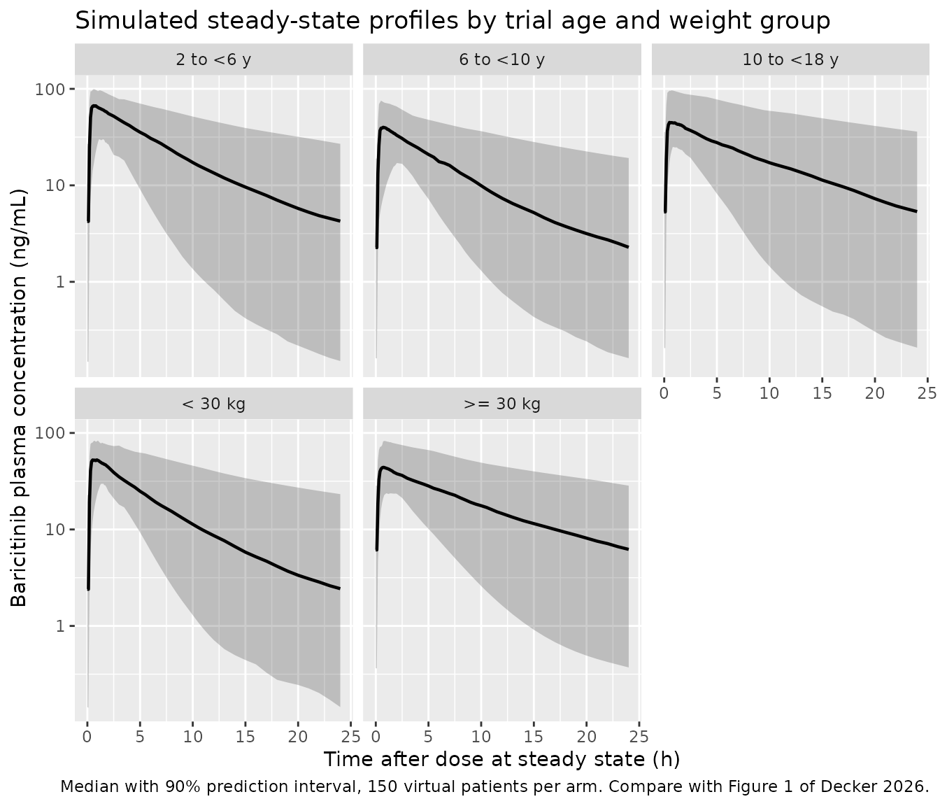
Figure 1 of Decker 2026 overlays observed pediatric concentrations from the open-label PK lead-in on the model-predicted median and 90% prediction interval for adults receiving 4 mg once daily. Observed data are not available, so the panels below show the simulated pediatric prediction interval for each arm at the dose it received.

sim |>
  mutate(time_after_dose = time - ss_start,
         treatment = factor(treatment, levels = arms$treatment)) |>
  group_by(treatment, time_after_dose) |>
  summarise(
    Q05 = quantile(Cc, 0.05, na.rm = TRUE),
    Q50 = quantile(Cc, 0.50, na.rm = TRUE),
    Q95 = quantile(Cc, 0.95, na.rm = TRUE),
    .groups = "drop"
  ) |>
  ggplot(aes(time_after_dose, Q50)) +
  geom_ribbon(aes(ymin = Q05, ymax = Q95), alpha = 0.25) +
  geom_line(linewidth = 0.8) +
  facet_wrap(~treatment) +
  scale_y_log10() +
  labs(
    x = "Time after dose at steady state (h)",
    y = "Baricitinib plasma concentration (ng/mL)",
    title = "Simulated steady-state profiles by trial age and weight group",
    caption = paste(
      "Median with 90% prediction interval,", n_per_arm,
      "virtual patients per arm. Compare with Figure 1 of Decker 2026."
    )
  )

Figures 2 and 3 - exposure versus weight band, and the 30 kg cut-off

Figure 2 plots simulated steady-state Cmax and AUC by weight range at 4 mg once daily against the adult 4 mg reference; Figure 3 repeats it under the proposed weight-based posology (2 mg below 30 kg, 4 mg at or above). Together they are the analysis that selected the 30 kg cut-off. The paper varied weight in 10 kg steps between 10 and 60 kg and in 20 kg steps between 60 and 120 kg, with eGFR fixed to the study range. The reproduction below uses those bands at both 2 mg and 4 mg.

bands <- tibble::tribble(
  ~band,        ~lo,  ~hi,
  "10-20 kg",    10,   20,
  "20-30 kg",    20,   30,
  "30-40 kg",    30,   40,
  "40-50 kg",    40,   50,
  "50-60 kg",    50,   60,
  "60-80 kg",    60,   80,
  "80-120 kg",   80,  120
) |>
  mutate(band = factor(band, levels = band))

grid <- tidyr::crossing(bands, amt_mg = c(2, 4)) |>
  mutate(arm = paste0(as.character(band), " | ", amt_mg, " mg"),
         id_offset = 100000L + 1000L * seq_len(dplyr::n()))

events_bands <- do.call(bind_rows, lapply(seq_len(nrow(grid)), function(i) {
  g <- grid[i, ]
  make_arm(
    n = 80L, amt_mg = g$amt_mg,
    wt_mean = (g$lo + g$hi) / 2, wt_lo = g$lo, wt_hi = g$hi,
    # eGFR fixed to the study range across all bands, per the paper's Methods.
    egfr_mean = 109, egfr_lo = 54.3, egfr_hi = 196,
    treatment = g$arm, id_offset = g$id_offset
  )
}))

stopifnot(anyDuplicated(events_bands[, c("id", "time", "evid")]) == 0L)
c(arms = nrow(grid), subjects = dplyr::n_distinct(events_bands$id))
#>     arms subjects 
#>       14     1120

sim_bands <- rxode2::rxSolve(
  mod, events = events_bands, keep = c("treatment", "WT")
) |>
  as.data.frame()

stopifnot(dplyr::n_distinct(sim_bands$id) == dplyr::n_distinct(events_bands$id))

exposure_bands <- sim_bands |>
  group_by(treatment, id) |>
  summarise(
    cmax_ss = max(Cc, na.rm = TRUE),
    # Linear-trapezoid AUC over the final dosing interval, for plotting only;
    # the validated NCA comparison below uses PKNCA.
    auc_ss  = sum(diff(time) * (head(Cc, -1) + tail(Cc, -1)) / 2, na.rm = TRUE),
    .groups = "drop"
  ) |>
  tidyr::separate(treatment, into = c("band", "dose_label"), sep = " \\| ",
                  remove = FALSE) |>
  mutate(band = factor(band, levels = levels(bands$band)))

# Adult AD reference at 4 mg QD (Decker 2026 Table 2, adult AD column).
adult_ref <- tibble(metric = c("Cmax,ss (ng/mL)", "AUCtau,ss (ng*h/mL)"),
                    value  = c(45.0, 380))

exposure_bands |>
  tidyr::pivot_longer(c(cmax_ss, auc_ss), names_to = "metric") |>
  mutate(metric = ifelse(metric == "cmax_ss",
                         "Cmax,ss (ng/mL)", "AUCtau,ss (ng*h/mL)")) |>
  ggplot(aes(band, value, fill = dose_label)) +
  geom_boxplot(outlier.size = 0.4) +
  geom_hline(data = adult_ref, aes(yintercept = value),
             linetype = "dashed", colour = "red") +
  facet_wrap(~metric, scales = "free_y", ncol = 1) +
  labs(
    x = "Weight band", y = NULL, fill = "Dose",
    title = "Simulated steady-state exposure by weight band and dose",
    caption = paste(
      "Red dashed line: exposure in adult patients with AD at 4 mg QD",
      "(Table 2). Compare with Figures 2 and 3 of Decker 2026."
    )
  ) +
  theme(axis.text.x = element_text(angle = 30, hjust = 1))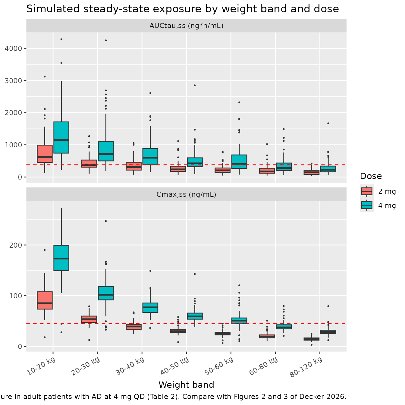

The reproduction supports the paper’s reasoning and its 30 kg cut-off. At 2 mg the 10-20 kg and 20-30 kg bands bracket the adult AUC reference, while from 30 kg upward 2 mg falls short and 4 mg is required. The paper’s own numbers for the resulting posology are that Cmax runs 12% above the adult value at or above 30 kg and 27% above below 30 kg, with AUC closely matched; the same asymmetry - AUC matched, Cmax somewhat high in the lightest band - is visible here. The paper’s stated reason for preferring AUC matching is that the adult exposure-response analysis found Cmax not to be a relevant driver of efficacy or safety.

# Quantify the cut-off argument: which dose puts each band's median AUC closest
# to the adult 4 mg reference of 380 ng*h/mL?
exposure_bands |>
  group_by(band, dose_label) |>
  summarise(median_auc = median(auc_ss), .groups = "drop") |>
  mutate(`% of adult AUC` = 100 * median_auc / 380) |>
  tidyr::pivot_wider(id_cols = band, names_from = dose_label,
                     values_from = `% of adult AUC`) |>
  dplyr::rename("Weight band" = band) |>
  knitr::kable(
    digits  = 0,
    caption = paste(
      "Median simulated AUC(tau,ss) as a percentage of the adult 4 mg AUC",
      "of 380 ng*h/mL, by weight band and dose."
    )
  )

Median simulated AUC(tau,ss) as a percentage of the adult 4 mg AUC of 380 ng*h/mL, by weight band and dose.
Weight band	2 mg	4 mg
10-20 kg	164	302
20-30 kg	98	188
30-40 kg	81	158
40-50 kg	62	112
50-60 kg	54	107
60-80 kg	45	74
80-120 kg	39	59

PKNCA validation

sim_nca <- sim |>
  filter(!is.na(Cc)) |>
  select(id, time, Cc, treatment)

# Guarantee a record at the interval start (the pre-dose trough) so PKNCA does
# not warn about an AUC range starting before the first measurement.
sim_nca <- bind_rows(
  sim_nca,
  sim_nca |> distinct(id, treatment) |> mutate(time = ss_start, Cc = 0)
) |>
  distinct(id, treatment, time, .keep_all = TRUE) |>
  arrange(id, treatment, time)

dose_df <- events |>
  filter(evid == 1) |>
  select(id, time, amt, treatment)

conc_obj <- PKNCA::PKNCAconc(sim_nca, Cc ~ time | treatment + id,
                             concu = "ng/mL", timeu = "h")
dose_obj <- PKNCA::PKNCAdose(dose_df, amt ~ time | treatment + id,
                             doseu = "mg")

# Steady-state interval: the final dosing interval.
intervals <- data.frame(
  start   = ss_start,
  end     = ss_start + tau,
  cmax    = TRUE,
  tmax    = TRUE,
  cmin    = TRUE,
  auclast = TRUE,
  cav     = TRUE
)

nca_res <- PKNCA::pk.nca(
  PKNCA::PKNCAdata(conc_obj, dose_obj, intervals = intervals)
)

Comparison against published NCA

auclast over the final dosing interval is the model’s AUC(tau,ss) and cmax is Cmax,ss. All five arms are valid targets, since Table 2’s exposure columns reconcile with their own clearances (checked above).

published <- tibble::tribble(
  ~treatment,     ~cmax, ~auclast,
  "2 to <6 y",     64.8,      298,
  "6 to <10 y",    45.7,      279,
  "10 to <18 y",   50.7,      383,
  "< 30 kg",       57.1,      298,
  ">= 30 kg",      50.3,      383
)

cmp <- nlmixr2lib::ncaComparisonTable(
  simulated     = nca_res,
  reference     = published,
  by            = "treatment",
  units         = c(cmax = "ng/mL", auclast = "ng*h/mL"),
  tolerance_pct = 20
)

knitr::kable(
  cmp,
  caption = paste(
    "Simulated versus published steady-state exposure (Decker 2026 Table 2).",
    "* differs from the reference by more than 20%."
  ),
  align = c("l", "l", "r", "r", "r")
)

Simulated versus published steady-state exposure (Decker 2026 Table 2). * differs from the reference by more than 20%.
NCA parameter	treatment	Reference	Simulated	% diff
Cmax (ng/mL)	2 to <6 y	64.8	76	+17.2%
Cmax (ng/mL)	6 to <10 y	45.7	45.1	-1.3%
Cmax (ng/mL)	10 to <18 y	50.7	48.8	-3.8%
Cmax (ng/mL)	< 30 kg	57.1	59.3	+3.9%
Cmax (ng/mL)	>= 30 kg	50.3	48.3	-4.0%
AUClast (ng*h/mL)	2 to <6 y	298	502	+68.6%*
AUClast (ng*h/mL)	6 to <10 y	279	296	+6.1%
AUClast (ng*h/mL)	10 to <18 y	383	432	+12.7%
AUClast (ng*h/mL)	< 30 kg	298	336	+12.7%
AUClast (ng*h/mL)	>= 30 kg	383	445	+16.2%

differs from reference by more than ±20%.

Cmax reproduces closely in the arms that carry the dosing recommendation. AUC is over-predicted, by the smallest margin in the largest, best-determined arms and by more in the lightest ones. The pattern is the mirror image of the clearance residual diagnosed in the structural check, and has the same three compounding causes, none of them a transcription choice:

AUC = Dose / (CL/F), so the clearance under-prediction reappears as an AUC over-prediction of the same relative size. The driver is the published model’s fixed 0.75 allometric exponent; the paper’s own estimated-exponent analysis returned 0.59, and substituting it closes the gap on both weight-group arms to under 4% (see the diagnostic table above).
The simulated summaries are geometric means over a weight distribution, while the typical-value calculation uses the mean weight. Because WT^0.75 is concave, the geometric-mean clearance over a spread of weights falls below the clearance at the mean weight, adding a few percent more AUC. The effect is largest in the widest arms.
The one starred row, 2 to <6 y AUC at +68.6%, is compared against the least precise cell in Table 2. As shown above, the three dose cells of that age group share the same reported weight and eGFR yet span a factor of 1.34 in published CL/F; the 2 mg cell used here is the extreme of that spread, and the model sits only -9.9% and -15.1% against the group’s other two cells. It is context rather than a firm target.

No parameter was adjusted to improve any of these comparisons.

Assumptions and deviations

The between-subject variances come from ESM Table S2, not from Table 1’s %CV column. The paper reports the BSV twice and the two reports disagree for CLnr/F and CLr/F. Table S2 tabulates the OMEGA variances directly; their square roots reproduce Table S2’s own printed SD diagonal for all six terms, its RSE% column matches Table 1’s %SEE column for all six, and its correlations combined with those SDs reproduce Table 1’s two covariances. Table 1’s %CV column back-transforms to Table S2 for D1, V1/F, Q and V2/F but not for CLnr/F (58.4% implies 0.293 versus 0.313) or CLr/F (62.3% implies 0.328 versus 0.358). Decisively, reconstructing the covariance block from Table 1’s %CV values while keeping Table 1’s own covariances yields a matrix with a negative eigenvalue (-0.0073) - an impossible covariance matrix - while the Table S2 variances give a positive definite block (minimum eigenvalue 0.0038). Both reconstructions are computed live in the Source trace section.
cov(CLnr/F, V1/F) is fixed to zero. Table 1 reports covariances for the CLnr/F-CLr/F and CLr/F-V1/F pairs only. ESM Table S2 resolves the third element explicitly, printing corr(CLnr, V1) = 0.00, so it is encoded as fixed(0) rather than estimated or inferred.
Weight and eGFR distributions are reconstructed, not observed. Individual covariates are not published. Each arm’s weight and baseline eGFR are drawn from truncated normals matched to the mean and min/max reported in Table 2 and Table S1. The true distributions are skewed within groups, so the simulated exposure spread will not match the published CV% exactly.
The weight-group arms use Table 2’s weight statistics, not Table S1’s. Table S1’s <30 kg and >=30 kg columns cover all 88 and 304 patients in those strata, whereas Table 2 footnote d restricts its weight-group columns to the 35 and 106 patients who received the dose the weight-based posology would assign. Since the exposure targets come from Table 2, its weight statistics (21.5 and 56.9 kg) are the matching ones. Baseline eGFR is unavailable for the restricted subset, so Table S1’s stratum means (125 and 105) are used.
The time-varying eGFR arm is switched off. The model carries the Wahlby 2004 baseline/difference decomposition of eGFR, but the paper reports no on-treatment eGFR trajectory and no distribution for the change from baseline. All simulations here set CRCL = CRCL_BASE, so the delta term contributes nothing and renal clearance scales only with baseline eGFR. Users with longitudinal eGFR data should populate both columns.
Simulated AUC runs above Table 2, most in the lightest arms. This is a property of the published fixed-exponent model as encoded, not an unresolved transcription question: the structural check localises it to clearance, and the paper’s own estimated-exponent sensitivity analysis (0.59 rather than the fixed 0.75) accounts for it, bringing both weight-group arms to the same residual of under 4%. Nothing was tuned to reduce it.
Allometric exponents are the fixed values, not the estimated ones. The Discussion reports a sensitivity analysis in which the exponents were estimated rather than fixed, returning 0.59 for clearance-related and 0.66 for volume-related parameters. Those are explicitly not the final model - Table 1 reports 0.75 and 1 with FIX - so only the fixed values are encoded. The 0.59 exponent appears in this vignette solely as a diagnostic explaining the clearance residual, and the paper notes that the weight-based dose recommendation is unchanged either way.
Half-life is computed analytically, not by NCA. The Table 2 t1/2 values derive from post-hoc individual parameters. Estimating a terminal half-life by regression within a single 24 h steady-state interval is biased when the half-life is 11-17 h, so the structural comparison uses the analytic two-compartment terminal (beta) half-life and half.life is omitted from the PKNCA interval specification.
No exposure-response model is encoded. The paper’s E-R analysis (Figures 4 and 5, Figure S5) summarises observed vIGA-AD 0/1 response rates by steady-state average-concentration quartile and by weight or age subgroup. It reports no fitted E-R parameters, so there is nothing to encode; the logistic regressions behind Figure S5 are reported only as significance markers.
Adult AD values are context, not model content. The adult exposures quoted (AUC(tau,ss) 380 ng*h/mL, Cmax,ss 45.0 ng/mL) come from Table 2 and are used only as a reference line. The adult AD model itself is a separate publication and is not encoded here.
No covariate beyond weight and renal function is in the model. Age, sex and race were screened by stepwise covariate modeling and none met the forward-inclusion criteria (p <= 0.01 and a >= 5% reduction in the relevant BSV), so backward exclusion was never run and the base model became the final model. The screened-but-excluded covariates are recorded in the model file’s covariatesDataExcluded metadata.
The blood-to-plasma conversion is upstream of the model. Lead-in whole-blood microsamples were multiplied by 1.32 before modeling; the model operates on plasma-equivalent concentrations only.
Mis-recorded dose times were retained by the authors. The Discussion notes clusters of implausible concentrations at ~4 h and ~24 h post-dose, attributed to incorrect recording of time from dose rather than to disposition. A sensitivity refit excluding them changed the estimates minimally, so they were kept in the final analysis; the packaged parameters are therefore the all-data estimates.