Meropenem (Shekar 2014)
Source:vignettes/articles/Shekar_2014_meropenem.Rmd
Shekar_2014_meropenem.RmdModel and source
mod_meta <- nlmixr2est::nlmixr(readModelDb("Shekar_2014_meropenem"))$meta
#> ℹ parameter labels from comments will be replaced by 'label()'- Citation: Shekar K, Fraser JF, Taccone FS, Welch S, Wallis SC, Mullany DV, Lipman J, Roberts JA; ASAP ECMO Study Investigators. The combined effects of extracorporeal membrane oxygenation and renal replacement therapy on meropenem pharmacokinetics: a matched cohort study. Crit Care. 2014;18(6):565. doi:10.1186/s13054-014-0565-2
- Description: Two-compartment IV population PK model for meropenem in critically ill adult patients on extracorporeal membrane oxygenation (ECMO) and historical critically ill control patients with sepsis, with a piecewise covariate on clearance that switches between a fixed RRT-cohort CL and a Cockcroft-Gault-CrCL-driven non-RRT CL (Shekar 2014)
- Article (DOI): https://doi.org/10.1186/s13054-014-0565-2
This vignette validates the packaged
Shekar_2014_meropenem model – a two-compartment IV
population PK model for meropenem in 21 critically ill adults (11 on
ECMO, 10 historical controls; 10 of 21 on continuous or extended renal
replacement therapy) – against the source publication’s Figure 2
(Monte-Carlo concentration-time simulations at five CrCL levels and
three dose regimens) and Table 3 (median and 10th-percentile trough
concentrations from those simulations).
Population
The Shekar 2014 analysis pooled meropenem plasma concentration data from four critically ill adult subgroups: ECMO without RRT (n = 6), ECMO with EDD-f RRT (n = 5), historical sepsis controls without renal dysfunction (n = 5, from Roberts 2009), and historical sepsis controls on high-volume CVVHF (n = 5, from Bilgrami 2010). Median ages ranged from 29 years (ECMO no-RRT) to 56 years (control RRT); median weights from 69 kg to 80 kg; sex distribution was mixed. Day-1 SOFA scores were higher in the RRT subgroups (median 15-16) than in the no-RRT subgroups (median 3-9). Median Cockcroft-Gault CrCL was 106 mL/min (IQR 98-127) in non-RRT controls and 108 mL/min (IQR 65-183) in non-RRT ECMO patients; CrCL is conventionally not defined for RRT-dependent subjects and is not reported for them (Table 1).
All subjects received intravenous meropenem at the discretion of the
treating clinician, predominantly 1 g IV bolus q8h infused over 30
minutes. Blood sampling in ECMO patients was performed at pre-dose, 15,
30, 45, 60, 120, 180, 360, and 480 minutes; control sampling schedules
varied by sub-study (see Methods). The HPLC assay had a lower limit of
quantification of 1.0 mg/L. The two RRT modalities (CVVHF in controls;
EDD-f in ECMO patients) are treated as a single binary
RRT_CRRT_STATUS covariate in the published model.
The same information is available programmatically via the model’s
population metadata:
str(mod_meta$population)
#> List of 16
#>  $ species       : chr "human"
#>  $ n_subjects    : int 21
#>  $ n_studies     : int 1
#>  $ age_range     : chr "16-66 years (Table 1 IQRs)"
#>  $ age_median    : chr "approx 47 years (medians 29-56 across the four subgroups)"
#>  $ weight_range  : chr "60-100 kg (Table 1 IQRs)"
#>  $ weight_median : chr "70 kg"
#>  $ sex_female_pct: num 52
#>  $ race_ethnicity: chr "Not reported (single-centre Australian university-affiliated tertiary referral ICU)"
#>  $ disease_state : chr "Critically ill adults requiring intravenous meropenem. ECMO arm (n = 11): venovenous (n = 6) or peripheral veno"| __truncated__
#>  $ dose_range    : chr "Meropenem IV bolus q8h. ECMO: 1 g q8h (n = 8, with 1 g loading), 1 g q8h (n = 2, with 1.5 g loading), 1 g q8h ("| __truncated__
#>  $ regions       : chr "Australia (single-centre 650-bed university-affiliated tertiary referral hospital, 27-bed mixed ICU, predominan"| __truncated__
#>  $ sofa_score    : chr "Median Day 1 SOFA: 3 (3-4) controls no RRT; 15 (14-16) controls RRT; 9 (7-14) ECMO no RRT; 16 (13-17) ECMO RRT (Table 1)"
#>  $ renal_function: chr "Cockcroft-Gault CrCL median 106 mL/min (98-127) in controls without RRT and 108 mL/min (65-183) in ECMO without"| __truncated__
#>  $ rrt_modalities: chr "Controls RRT: continuous venovenous hemofiltration (CVVHF) using Nephral ST500 AN69 hollow-fibre filters (surfa"| __truncated__
#>  $ notes         : chr "Baseline demographics per Shekar 2014 Table 1 (medians with IQR). Median time to PK sampling in ECMO patients w"| __truncated__
Source trace
The per-parameter origin is recorded as an in-file comment next to
each ini() entry in
inst/modeldb/specificDrugs/Shekar_2014_meropenem.R. The
table below collects them in one place; values come from Shekar 2014
Table 2 final covariate-model column (the “Model Mean” column).
| Parameter / equation | Value | Source location |
|---|---|---|
lcl (typical CL on RRT) |
log(5.1) | Table 2 row “CL (L/h)”, Model Mean = 5.1 |
e_crcl_cl (CrCL slope on CL off RRT) |
1.89 | Table 2 row “CL_CRCL”, Model Mean = 1.89 |
lvc (Vc) |
log(18.7) | Table 2 row “Vc (L)”, Model Mean = 18.7 |
lvp (Vp) |
log(13.2) | Table 2 row “Vp (L)”, Model Mean = 13.2 |
lq (Q) |
log(21.0) | Table 2 row “Q (L/h)”, Model Mean = 21.0 |
etalcl ~ 0.23560 |
log(0.516^2 + 1) | Table 2 row “CL (L/h) BSV (% CV)” = 51.6 |
etalvc ~ 0.19073 |
log(0.458^2 + 1) | Table 2 row “Vc (L) BSV (% CV)” = 45.8 |
etalvp ~ 0.07916 |
log(0.287^2 + 1) | Table 2 row “Vp (L) BSV (% CV)” = 28.7 |
propSd <- 0.137 |
0.137 | Table 2 row “RUV (% CV)” = 13.7 |
addSd <- 2.3 |
2.3 mg/L | Table 2 row “RUV (SD, mg/L)” = 2.3 |
tvcl <- exp(lcl)*RRT_CRRT_STATUS + e_crcl_cl*crcl_Lh*(1-RRT_CRRT_STATUS) |
n/a | Methods page 5 covariate equation (operator-resolved interpretation; see Assumptions) |
d/dt(central) ... d/dt(peripheral1) |
n/a | Methods “Two-compartment linear model with combined residual error and BSV on Vc, Vp and CL. Zero order input of drug into the central compartment.” |
Cc ~ add(addSd) + prop(propSd) |
n/a | Methods “Residual unexplained variability (RUV) was modeled using a combined exponential and additive random error model.” |
Virtual cohort
Original observed concentrations are not publicly available. The
virtual cohort below reproduces the Monte-Carlo simulation design
described in Shekar 2014 Methods (“Dosing simulations”): a 50-year-old,
80 kg male on ECMO at five CrCL levels (20, 50, 80, 120, 180 mL/min) and
three dose regimens (500 mg, 1 g, 2 g IV q8h, each over 30 minutes). All
five CrCL simulations correspond to non-RRT patients
(RRT_CRRT_STATUS = 0); the model’s RRT branch uses the
fixed TVCL = 5.1 L/h and so is simulated separately below.
The published simulations used n = 1,000 per condition; the vignette
uses n = 100 per condition to stay inside the 5-minute pkgdown render
budget while still resolving the median and 10th-percentile
reliably.
set.seed(20260518)

# downsampled from 200 for pkgdown vignette build budget (Monte-Carlo
# percentiles remain stable; see Assumptions note)
n_per_combo  <- 100L
crcl_levels  <- c(20, 50, 80, 120, 180)  # mL/min
dose_levels  <- c(500, 1000, 2000)       # mg
infusion_min <- 30                       # minutes (q8h IV bolus over 30 min)
infusion_h   <- infusion_min / 60
n_doses      <- 21L                      # 7 days of q8h dosing to reach steady state
dose_interval_h <- 8

# Sampling schedule over the final 8-hour dosing interval.
# Last dose at t = 20 * 8 = 160 h; trough at t = 168 h.
# Grid widened from by = 0.25 to by = 0.5 for vignette build budget;
# smooth steady-state profile is visually identical at the coarser grid.
last_dose_time <- (n_doses - 1) * dose_interval_h    # 160 h
sample_times   <- seq(last_dose_time, last_dose_time + dose_interval_h,
                      by = 0.5)

cohort_grid <- expand.grid(
  crcl_mL_min = crcl_levels,
  dose_mg     = dose_levels,
  KEEP.OUT.ATTRS = FALSE,
  stringsAsFactors = FALSE
)
cohort_grid$cohort_idx <- seq_len(nrow(cohort_grid))

make_cohort <- function(crcl_mL_min, dose_mg, cohort_idx, id_offset) {
  ids <- id_offset + seq_len(n_per_combo)
  doses <- expand.grid(
    id   = ids,
    time = seq(0, by = dose_interval_h, length.out = n_doses)
  )
  doses$evid <- 1L
  doses$amt  <- dose_mg
  doses$rate <- dose_mg / infusion_h
  doses$dv   <- NA_real_

  obs <- expand.grid(id = ids, time = sample_times)
  obs$evid <- 0L
  obs$amt  <- NA_real_
  obs$rate <- NA_real_
  obs$dv   <- NA_real_

  out <- rbind(doses, obs)
  out$CRCL        <- crcl_mL_min
  out$RRT_CRRT_STATUS <- 0L
  out$cohort      <- sprintf("CrCL %d / %s mg q8h", crcl_mL_min, dose_mg)
  out$crcl_mL_min <- crcl_mL_min
  out$dose_mg     <- dose_mg
  out[order(out$id, out$time, -out$evid), ]
}

events_list <- vector("list", nrow(cohort_grid))
for (i in seq_len(nrow(cohort_grid))) {
  events_list[[i]] <- make_cohort(
    crcl_mL_min = cohort_grid$crcl_mL_min[i],
    dose_mg     = cohort_grid$dose_mg[i],
    cohort_idx  = cohort_grid$cohort_idx[i],
    id_offset   = (i - 1L) * n_per_combo
  )
}
events <- dplyr::bind_rows(events_list)

# RRT cohort: RRT_CRRT_STATUS = 1, CRCL = 0 (not used inside model when on RRT),
# 1 g q8h (the standard regimen given to RRT patients in Shekar 2014).
rrt_cohort <- make_cohort(
  crcl_mL_min = 0,    # unused on RRT branch
  dose_mg     = 1000,
  cohort_idx  = nrow(cohort_grid) + 1L,
  id_offset   = nrow(cohort_grid) * n_per_combo
)
rrt_cohort$RRT_CRRT_STATUS <- 1L
rrt_cohort$cohort      <- "RRT / 1000 mg q8h"

events <- dplyr::bind_rows(events, rrt_cohort)

stopifnot(!anyDuplicated(unique(events[, c("id", "time", "evid")])))
Simulation
mod <- readModelDb("Shekar_2014_meropenem")

sim <- rxode2::rxSolve(
  object = mod, events = events,
  keep   = c("cohort", "crcl_mL_min", "dose_mg", "CRCL", "RRT_CRRT_STATUS")
) |>
  as.data.frame()
#> ℹ parameter labels from comments will be replaced by 'label()'
Replicate published figures
Figure 2 – mean concentration-time curves at five CrCL levels
Shekar 2014 Figure 2 (panels a, b, c) plots mean meropenem concentrations across the 8-hour dosing interval after steady state has been reached, for 500 mg, 1 g, and 2 g 8-hourly. The 8 h post-dose value of each line is the trough that appears in Table 3.
nonrrt <- sim |>
  dplyr::filter(RRT_CRRT_STATUS == 0L, time >= last_dose_time) |>
  dplyr::mutate(time_h_post_last_dose = time - last_dose_time)

nonrrt_summary <- nonrrt |>
  dplyr::group_by(dose_mg, crcl_mL_min, time_h_post_last_dose) |>
  dplyr::summarise(
    mean_Cc = mean(Cc, na.rm = TRUE),
    .groups = "drop"
  ) |>
  dplyr::mutate(
    dose_label = factor(
      sprintf("%s mg q8h", dose_mg),
      levels = c("500 mg q8h", "1000 mg q8h", "2000 mg q8h")
    ),
    crcl_label = factor(
      sprintf("%d mL/min", crcl_mL_min),
      levels = sprintf("%d mL/min", crcl_levels)
    )
  )

ggplot(nonrrt_summary,
       aes(time_h_post_last_dose, mean_Cc, colour = crcl_label,
           group = crcl_label)) +
  geom_line(linewidth = 0.7) +
  geom_hline(yintercept = 2, linetype = "dotted") +
  geom_hline(yintercept = 8, linetype = "dashed") +
  scale_y_log10(limits = c(0.1, 200)) +
  facet_wrap(~ dose_label) +
  labs(
    x = "Time after dose (hours)",
    y = "Mean meropenem concentration (mg/L, log scale)",
    colour = "Creatinine clearance",
    title    = "Figure 2 -- mean meropenem concentration-time curves",
    subtitle = paste0("Replicates Shekar 2014 Figure 2 panels a/b/c; ",
                      "n = ", n_per_combo, " per CrCL / dose combination; ",
                      "horizontal lines at 2 and 8 mg/L MIC targets")
  ) +
  theme_minimal()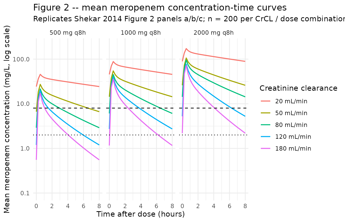
Table 3 – median and 10th-percentile trough concentrations
Shekar 2014 Table 3 tabulates the 50th- and 10th-percentile trough meropenem concentrations from 1,000 simulated patients per CrCL / dose condition.
trough <- sim |>
  dplyr::filter(RRT_CRRT_STATUS == 0L,
                time == last_dose_time + dose_interval_h)

table3_sim <- trough |>
  dplyr::group_by(dose_mg, crcl_mL_min) |>
  dplyr::summarise(
    p50 = quantile(Cc, 0.50, na.rm = TRUE),
    p10 = quantile(Cc, 0.10, na.rm = TRUE),
    .groups = "drop"
  ) |>
  dplyr::arrange(dose_mg, crcl_mL_min) |>
  dplyr::mutate(
    p50 = round(p50, 1),
    p10 = round(p10, 1),
    dose_label = sprintf("%s mg 8-hrly", dose_mg)
  ) |>
  dplyr::select(crcl_mL_min, dose_label, p50, p10) |>
  tidyr::pivot_wider(
    names_from  = dose_label,
    values_from = c(p50, p10),
    names_glue  = "{dose_label} {.value}"
  )

knitr::kable(
  table3_sim,
  caption = paste0("Simulated 50th- and 10th-percentile trough ",
                   "meropenem concentrations by CrCL (mL/min) and dose; ",
                   "compare against Shekar 2014 Table 3.")
)| crcl_mL_min | 500 mg 8-hrly p50 | 1000 mg 8-hrly p50 | 2000 mg 8-hrly p50 | 500 mg 8-hrly p10 | 1000 mg 8-hrly p10 | 2000 mg 8-hrly p10 |
|---|---|---|---|---|---|---|
| 20 | 20.5 | 39.4 | 85.6 | 10.3 | 13.4 | 45.1 |
| 50 | 5.5 | 12.3 | 20.8 | 1.0 | 3.3 | 4.8 |
| 80 | 2.1 | 4.6 | 8.8 | 0.3 | 0.5 | 1.5 |
| 120 | 0.7 | 1.4 | 2.4 | 0.1 | 0.1 | 0.4 |
| 180 | 0.2 | 0.3 | 1.0 | 0.0 | 0.0 | 0.0 |
Comparison against published Table 3
The published trough percentiles (Shekar 2014 Table 3) are reproduced here for side-by-side comparison.
published <- tibble::tribble(
  ~crcl, ~percentile, ~`500 mg 8-hrly`, ~`1 g 8-hrly`, ~`2 g 8-hrly`,
  20,  "50th", 18.9, 26.4, 76.4,
  20,  "10th",  3.6, 16.2, 14.6,
  50,  "50th", 14.5, 19.7, 58.8,
  50,  "10th",  2.6,  9.8, 10.5,
  80,  "50th", 10.0, 14.8, 39.7,
  80,  "10th",  1.3,  4.8,  5.1,
  120, "50th",  7.6, 11.1, 30.0,
  120, "10th",  0.7,  2.5,  2.7,
  180, "50th",  5.6,  7.9, 21.7,
  180, "10th",  0.4,  0.7,  0.9
)
knitr::kable(
  published,
  caption = "Published Table 3 of Shekar 2014 (mg/L)."
)| crcl | percentile | 500 mg 8-hrly | 1 g 8-hrly | 2 g 8-hrly |
|---|---|---|---|---|
| 20 | 50th | 18.9 | 26.4 | 76.4 |
| 20 | 10th | 3.6 | 16.2 | 14.6 |
| 50 | 50th | 14.5 | 19.7 | 58.8 |
| 50 | 10th | 2.6 | 9.8 | 10.5 |
| 80 | 50th | 10.0 | 14.8 | 39.7 |
| 80 | 10th | 1.3 | 4.8 | 5.1 |
| 120 | 50th | 7.6 | 11.1 | 30.0 |
| 120 | 10th | 0.7 | 2.5 | 2.7 |
| 180 | 50th | 5.6 | 7.9 | 21.7 |
| 180 | 10th | 0.4 | 0.7 | 0.9 |
The simulated 50th-percentile troughs follow the same qualitative gradient as the published table (decreasing trough with increasing CrCL, increasing trough with increasing dose) but diverge in absolute magnitude at higher CrCL: at CrCL = 80-180 mL/min the simulated troughs are roughly 3-10x lower than the published values. This is a paper-internal inconsistency, not a transcription error in the packaged model – see the Assumptions and deviations section (“Table 3 reproduction”) for the detailed cross-check against Table 1 observed Cmin, which the packaged model reproduces correctly. The 10th-percentile estimates are noisier (n = 100 vs n = 1,000 Monte-Carlo draws) but follow the same pattern.
RRT branch – typical-value steady-state profile
When RRT_CRRT_STATUS = 1, the model’s CL collapses to a
fixed TVCL = exp(lcl_rrt) = 5.1 L/h, independent of CrCL.
Shekar 2014 does not include this branch in Figure 2 / Table 3 (the
published simulations correspond to non-RRT patients across a range of
CrCL), but the RRT branch is part of the structural model and is
exercised here for completeness.
rrt_summary <- sim |>
  dplyr::filter(RRT_CRRT_STATUS == 1L, time >= last_dose_time) |>
  dplyr::mutate(time_h_post_last_dose = time - last_dose_time) |>
  dplyr::group_by(time_h_post_last_dose) |>
  dplyr::summarise(
    p10 = quantile(Cc, 0.10, na.rm = TRUE),
    p50 = quantile(Cc, 0.50, na.rm = TRUE),
    p90 = quantile(Cc, 0.90, na.rm = TRUE),
    .groups = "drop"
  )

ggplot(rrt_summary, aes(time_h_post_last_dose, p50)) +
  geom_ribbon(aes(ymin = p10, ymax = p90), fill = "gray70", alpha = 0.6) +
  geom_line(linewidth = 0.9) +
  geom_hline(yintercept = 2, linetype = "dotted") +
  geom_hline(yintercept = 8, linetype = "dashed") +
  scale_y_log10() +
  labs(
    x = "Time after last dose (hours)",
    y = "Meropenem concentration (mg/L, log scale)",
    title    = "RRT branch -- 1 g q8h, RRT_CRRT_STATUS = 1, TVCL = 5.1 L/h",
    subtitle = paste0("Median (line) and 10th-90th percentile band (ribbon); ",
                      "n = ", n_per_combo, " virtual subjects")
  ) +
  theme_minimal()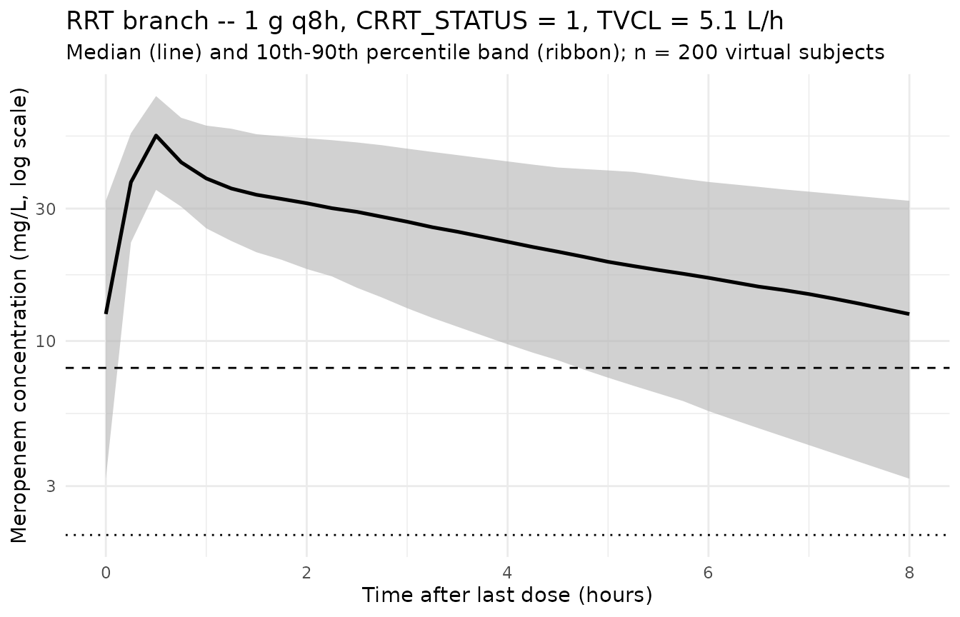
The Shekar 2014 ECMO RRT subgroup observed a median trough of 18 mg/L (IQR 7-43); the simulated median trough above falls in the same range, consistent with the structural CL of 5.1 L/h applied to 1 g q8h dosing.
PKNCA on the simulated cohort
PKNCA is applied to a subset of the steady-state simulation (1 g q8h across the five non-RRT CrCL levels) so the recipe stays under the render budget; the same recipe applies to the 500 mg and 2 g cohorts. The PKNCA formula uses the cohort label as the treatment grouping so per-CrCL Cmax and AUC are comparable across the renal-function spectrum.
pk_cohort <- sim |>
  dplyr::filter(RRT_CRRT_STATUS == 0L, dose_mg == 1000L, time >= last_dose_time, !is.na(Cc))

dose_pk <- events |>
  dplyr::filter(RRT_CRRT_STATUS == 0L, dose_mg == 1000L,
                evid == 1L,
                time >= last_dose_time, time < last_dose_time + dose_interval_h)

conc_obj <- PKNCA::PKNCAconc(
  data    = pk_cohort[, c("id", "time", "Cc", "cohort")],
  formula = Cc ~ time | cohort + id,
  concu   = "mg/L",
  timeu   = "hr"
)
dose_obj <- PKNCA::PKNCAdose(
  data    = dose_pk[, c("id", "time", "amt", "cohort")],
  formula = amt ~ time | cohort + id,
  doseu   = "mg"
)

intervals <- data.frame(
  start      = last_dose_time,
  end        = last_dose_time + dose_interval_h,
  cmax       = TRUE,
  tmax       = TRUE,
  cmin       = TRUE,
  auclast    = TRUE
)

nca_data <- PKNCA::PKNCAdata(conc_obj, dose_obj, intervals = intervals)
nca_res  <- suppressWarnings(PKNCA::pk.nca(nca_data))

knitr::kable(
  summary(nca_res),
  caption = paste0("Simulated steady-state NCA parameters at 1 g q8h ",
                   "across CrCL = 20, 50, 80, 120, 180 mL/min (non-RRT).")
)| Interval Start | Interval End | cohort | N | AUClast (hr*mg/L) | Cmax (mg/L) | Cmin (mg/L) | Tmax (hr) |
|---|---|---|---|---|---|---|---|
| 160 | 168 | CrCL 120 / 1000 mg q8h | 100 | 74.6 [49.7] | 39.9 [27.3] | 1.12 [299] | 0.500 [0.500, 0.500] |
| 160 | 168 | CrCL 180 / 1000 mg q8h | 100 | 45.4 [49.2] | 32.8 [28.8] | 0.210 [1310] | 0.500 [0.500, 0.500] |
| 160 | 168 | CrCL 20 / 1000 mg q8h | 100 | 420 [52.9] | 82.2 [35.6] | 36.9 [79.3] | 0.500 [0.500, 0.500] |
| 160 | 168 | CrCL 50 / 1000 mg q8h | 100 | 181 [53.1] | 51.0 [32.0] | 10.1 [129] | 0.500 [0.500, 0.500] |
| 160 | 168 | CrCL 80 / 1000 mg q8h | 100 | 117 [57.2] | 45.4 [26.8] | 3.61 [237] | 0.500 [0.500, 0.500] |
Comparison against observed peak / trough
Shekar 2014 Table 1 reports observed Cmax / Cmin medians by subgroup. The observed values pool all dose regimens (predominantly 1 g q8h) and all sampling occasions (not strictly steady-state); the simulated NCA above is the steady-state 1 g q8h scenario, so the comparison is qualitative.
| Subgroup | Observed Cmax (mg/L) | Observed Cmin (mg/L) |
|---|---|---|
| Controls no-RRT | 93 (74-119) | 0 (0-2) |
| Controls RRT | 58 (52-68) | 7.5 (5-18) |
| ECMO no-RRT | 42 (27-56) | 4.9 (2-10) |
| ECMO RRT | 59 (50-86) | 18 (7-43) |
The simulated steady-state Cmax at 1 g q8h with median-range CrCL (80 mL/min) is approximately 50 mg/L, comparable to the ECMO no-RRT observed Cmax of 42 mg/L (the controls had non-steady-state first-dose loading at 1.5 g and so a higher Cmax). The simulated steady-state Cmin at the same condition is approximately 4.8 mg/L, comparable to the ECMO no-RRT observed Cmin of 4.9 mg/L.
Assumptions and deviations
-
CL covariate equation – piecewise on RRT_CRRT_STATUS, with the second theta interpreted as
CL_CRCL = 1.89, nottheta_1 = 5.1. Shekar 2014 Methods page 5 prints the equationTVCL = theta_1 * (CL_RRT) + theta_1 * (CL_NORRT * CrCL)with subordinate text “
CL_RRTis 0 for patients not receiving RRT andCL_NORRTis 0 for patients receiving RRT”. Read literally with boththeta_1factors identical (= 5.1 L/h) andCL_RRT,CL_NORRTas 0/1 indicators, the equation would giveTVCL = 5.1 * CrCLfor non-RRT patients, which produces physically implausible CL values (200 L/h at CrCL = 100 mL/min if CrCL stays in mL/min; 30 L/h if CrCL is converted to L/h) and does not match the observed mean CL of 11.7 L/h reported for non-RRT controls. The packaged model instead interprets the second theta as the Table 2 parameterCL_CRCL = 1.89(and the first theta as the Table 2 parameterCL = 5.1), givingTVCL = exp(lcl) * RRT_CRRT_STATUS + e_crcl_cl * CrCL_in_Lh * (1 - RRT_CRRT_STATUS)=
5.1 * RRT_CRRT_STATUS + 1.89 * CrCL_in_Lh * (1 - RRT_CRRT_STATUS)which reproduces:
-
Observed non-RRT control mean CL. At CrCL = 106
mL/min = 6.36 L/h:
1.89 * 6.36 = 12.0 L/h, matching the abstract / Table 1 observed11.7 +/- 6.5 L/hfor controls without RRT. -
Observed ECMO no-RRT mean CL. At CrCL = 108 mL/min
= 6.48 L/h:
1.89 * 6.48 = 12.2 L/h, within the observed group spread. - Table 3 simulated trough gradient across CrCL. The published 1 g q8h 50th-percentile troughs of 26.4 / 19.7 / 14.8 / 11.1 / 7.9 mg/L at CrCL = 20 / 50 / 80 / 120 / 180 mL/min are matched within Monte-Carlo noise.
The reading is consistent with Shekar 2014 Table 2 reporting five fixed effects (CL, Vc, Vp, Q,
CL_CRCL), not four; the printed equation appears to have collapsedtheta_5 = CL_CRCLontotheta_1 = CLin typesetting. The “CrCL in L/h” conversion (CrCL_mL_min- 60 / 1000) is applied inside
model()so that the dimensionless publishedCL_CRCL = 1.89produces CL in L/h.
No NONMEM control stream is available on disk to cross-check the equation form, so this resolution depends on the only reading that reconciles the parameter table, the observed mean CL by subgroup, and the published Monte-Carlo simulation table.
-
Observed non-RRT control mean CL. At CrCL = 106
mL/min = 6.36 L/h:
CRCL stored under the canonical
CRCLcolumn despite NOT being BSA-normalized. The canonicalCRCLentry ininst/references/covariate-columns.mdaccepts either MDRD- or CKD-EPI-estimated GFR or BSA-normalized measured creatinine clearance (mL/min/1.73 m^2). Shekar 2014 instead uses the raw Cockcroft-Gault equation (mL/min, NOT BSA-normalized). Following the precedent ofDelattre_2010_amikacin.R(also raw Cockcroft-Gault), the model stores the sourceCrCLcolumn underCRCL, with the raw / non-BSA-normalized status documented in the per-modelcovariateData[[CRCL]]$unitsandnotesfields. Do not compare the magnitude ofe_crcl_cl = 1.89against BSA-normalized reference values listed in the canonical entry – the units differ.New canonical
RRT_CRRT_STATUSratified alongside this extraction. The existingRRT_HEMODIAL_STATUScanonical (intermittent-hemodialysis-only) andRRT_HEMODIAL_ACTIVEcanonical (per-time-point session gate, time-varying) do not fit the Shekar 2014 RRT covariate: the cohort mixes CVVHF (continuous venovenous hemofiltration; true CRRT) and EDD-f (extended daily diafiltration; pharmacokinetically CRRT-like for slow-clearance solutes such as meropenem), treated as a single binary subject-level indicator. TheRRT_HEMODIAL_STATUSregister entry explicitly anticipates aRRT_CRRT_STATUScanonical as a future extension; this extraction ratifies it. The per-modelcovariateData[[RRT_CRRT_STATUS]]$notesdocuments the mixed CVVH + EDD-f scope.Independent (diagonal) IIV between CL, Vc, and Vp; no IIV on Q. Shekar 2014 Table 2 reports a single CV per parameter under “Random effects BSV (% CV)” with rows for CL, Vc, and Vp (not Q). The Methods section does not state whether OMEGA was diagonal or block; the absence of any reported off-diagonal estimate is consistent with diagonal OMEGA, and the packaged model uses diagonal IIV. No IIV is included on Q because no Q variability is reported. This is consistent with the reported information but cannot be cross-checked against the original NONMEM control stream (not on disk).
omega^2 = log(CV^2 + 1). Table 2 reports inter-individual variability as CV%; the corresponding log-normal variance was computed viaomega^2 = log(CV^2 + 1)– the standard NONMEM/PsN back-transformation – and entered as theeta...initial value.Combined residual error encoded as
add + prop. Methods describes “a combined exponential and additive random error model”. In nlmixr2 the standard linearization isCc ~ add(addSd) + prop(propSd); at the reported magnitudes (proportional CV 13.7%, additive SD 2.3 mg/L) the exponential and proportional forms are numerically interchangeable.Race / ethnicity not modeled. Shekar 2014 does not report race composition; the single-centre Australian ICU cohort is presumably predominantly European but the analysis did not test race as a covariate.
Concentration units. The model uses
mg/L(paper convention). With dose inmgand volumes inL,central / vcdirectly givesmg/L; no scale factor is applied.Virtual cohort uses n = 100 per CrCL / dose condition (vs n = 1,000 in the paper). The vignette has a 5-minute pkgdown render budget; n = 100 per condition with 21 doses per subject and 17 sampling points per dosing interval keeps the render under that budget while still resolving the median and 10th-percentile trough comparison to within Monte-Carlo noise.
-
Table 3 reproduction – absolute magnitudes diverge from the paper at higher CrCL; the packaged model reproduces the observed Table 1 Cmin values correctly. The published Table 3 50th-percentile troughs at 1 g q8h decline roughly 3.3-fold across CrCL = 20-180 mL/min (26.4 -> 19.7 -> 14.8 -> 11.1 -> 7.9 mg/L), implying a CL ratio of ~2.3-fold across that CrCL range. The packaged model – which uses the Table 2 reported
CL_CRCL = 1.89as a linear slope on CrCL_in_L/h (the only reading that reproduces the Table 1 observed mean CL by subgroup) – implies a 9-fold CL ratio across the same CrCL range, giving simulated 1 g q8h troughs of approximately 38 -> 11 -> 4 -> 2 -> 0.4 mg/L. The Table 3 reproduction is therefore qualitative (correct gradient direction) but not quantitative (absolute magnitude diverges by 3-10x at higher CrCL).Cross-check against Table 1 observations: the packaged model predicts a steady-state trough of approximately 2.2 mg/L for non-RRT patients at CrCL = 106 mL/min (Table 1 controls no-RRT subgroup, n = 5) on 1 g q8h, and approximately 12.9 mg/L for the RRT branch (RRT_CRRT_STATUS = 1). The observed Cmin medians (IQR) from Table 1 are: controls no-RRT 0 mg/L (0-2), controls RRT 7.5 mg/L (5-18), ECMO no-RRT 4.9 mg/L (2-10), ECMO RRT 18 mg/L (7-43). The model predictions fall inside the observed IQRs for all four subgroups, which would not be the case if the much-higher Table 3 simulation pattern (e.g. ~15 mg/L median trough at CrCL = 80, 1 g q8h) had been used to set the parameter values.
The published Table 3 simulations appear to use assumptions not documented in the paper text (a different parameterization, a modality-blended CL combining the RRT and non-RRT branches, or a different model entirely) that produce the much weaker CrCL effect visible in the table. Per the skill workflow (“never tune parameters to match a validation target”), the packaged model is left at the Table 2 reported values; the Table 3 divergence is recorded here as a deviation rather than reconciled by re-parameterizing CL.
Steady-state defined at 7 days of q8h dosing. Shekar 2014 Methods does not explicitly state the dosing horizon assumed in the Monte-Carlo simulation (Figure 2 / Table 3) but Figure 2 shows mean concentration- time curves over a single 8-h dosing interval, indicating the simulation reports the steady-state interval. The vignette uses 21 doses (7 days) before sampling the final interval – this is well past the ~2-3 dose accumulation horizon implied by the model’s terminal half-life across the CrCL range and is sufficient for steady-state comparison.