Ainuovirine population PK and exposure-response (Han 2024) • nlmixr2lib

Model and source

Han 2024 reports five fitted models, and this article packages all five: one population PK model and four univariate logistic exposure-response regressions (two endpoints, each fitted separately against two exposure metrics).

han_models <- c(
  "Han_2024_ainuovirine",
  "Han_2024_ainuovirine_virologic_ctrough",
  "Han_2024_ainuovirine_virologic_auctau",
  "Han_2024_ainuovirine_adr_ctrough",
  "Han_2024_ainuovirine_adr_auctau"
)

# readModelDb() returns the model FUNCTION; rxode2::rxode() resolves it to the
# ui exactly once so every downstream accessor ($population, $reference, ...)
# works. See pattern 7 of the skill's known-vignette-failure-patterns.
uis <- lapply(han_models, function(n) rxode2::rxode(readModelDb(n)))
#> ℹ parameter labels from comments will be replaced by 'label()'
names(uis) <- han_models

data.frame(
  Model = han_models,
  Role = c(
    "Population PK (2-compartment, first-order absorption + lag)",
    "Exposure-efficacy: HIV-RNA < 50 copies/mL at week 48 vs Ctrough",
    "Exposure-efficacy: HIV-RNA < 50 copies/mL at week 48 vs AUCtau",
    "Exposure-safety: any adverse drug reaction vs Ctrough",
    "Exposure-safety: any adverse drug reaction vs AUCtau"
  ),
  Source = c("Table 3", "Table 4 (upper)", "Table 4 (lower)",
             "Table 5 (upper)", "Table 5 (lower)")
) |>
  knitr::kable(caption = "The five models Han 2024 reports.", align = c("l", "l", "l"))

The five models Han 2024 reports.
Model	Role	Source
Han_2024_ainuovirine	Population PK (2-compartment, first-order absorption + lag)	Table 3
Han_2024_ainuovirine_virologic_ctrough	Exposure-efficacy: HIV-RNA < 50 copies/mL at week 48 vs Ctrough	Table 4 (upper)
Han_2024_ainuovirine_virologic_auctau	Exposure-efficacy: HIV-RNA < 50 copies/mL at week 48 vs AUCtau	Table 4 (lower)
Han_2024_ainuovirine_adr_ctrough	Exposure-safety: any adverse drug reaction vs Ctrough	Table 5 (upper)
Han_2024_ainuovirine_adr_auctau	Exposure-safety: any adverse drug reaction vs AUCtau	Table 5 (lower)

Citation: Han X, Sun J, Zhang Y, Jiang T, Zheng Q, Peng H, Wang Y, Xia W, Zhang T, Sun L, Yun X, Qin H, Wu H, Su B. Population pharmacokinetics of Ainuovirine and exposure-response analysis in human immunodeficiency virus-infected individuals. Chin Med J (Engl). 2024;137(20):2474-2482. doi:10.1097/CM9.0000000000002917.
Article: https://doi.org/10.1097/CM9.0000000000002917
PubMed Central: https://www.ncbi.nlm.nih.gov/pmc/articles/PMC11479413/

No supplementary material accompanies this article; every value below comes from the main text, its four tables, or its figure axes.

Ainuovirine (ANV) is a third-generation non-nucleoside reverse transcriptase inhibitor approved in China for HIV-1 infection. The headline pharmacological finding is that it is nonlinear in dose while linear in time-invariant disposition: dose-normalised exposure falls as the dose rises, but the elimination half-life is essentially the same at 75, 150 and 300 mg. Han 2024 therefore attributes the nonlinearity to absorption and carries it entirely in relative bioavailability rather than in a saturable elimination term.

Population

The population PK dataset pools two single-centre Chinese trials in antiretroviral-therapy-naive people living with HIV-1 (PLWH): ADYY-ACC007-103 (phase 1 multiple-ascending-dose; 75 mg n = 8, 150 mg n = 10, 300 mg n = 10; once daily for 10 days; rich sampling after the first and the last dose) and ADYY-ACC007-301 (phase 3; 150 mg once daily at bedtime on an empty stomach for 48 weeks; n = 309; sparse sampling at weeks 12, 24, 36 and 48). Of 341 participants who took ANV, 4 whose concentrations were all below the limit of quantification were dropped, leaving 337 subjects and 1947 plasma concentrations (Han 2024 Results, Tables 1 and 2).

The cohort is young (mean age 31.2 years, SD 9.8; range 18-61 per the Discussion), predominantly male (319/337, 94.7%), and of near-normal body habitus (mean weight 66.9 kg SD 11.2; mean BMI 22.56 kg/m^2 SD 3.19). Baseline hepatic and renal laboratory values are unremarkable (mean ALT 26.5 IU/L, AST 23.6 IU/L, albumin 47.1 g/L, creatinine clearance 78.1 mL/min).

No covariate reached significance. Age, sex, weight, height, BMI, ALT, AST, total bilirubin, albumin, creatinine, creatinine clearance, total cholesterol and combination medication were all screened and rejected, so Han 2024’s base model is its final model. Age alone produced a significant OFV drop but was discarded because its coefficient was -0.00625 (essentially zero) and it reduced the CL random effect by only 0.7%. The paper is explicit that this null result is bounded by the design rather than being a general statement about ANV: the age range is narrow, only 18 of 337 subjects were female, and few participants with hepatic or renal impairment were enrolled. The screened-but-rejected covariates are preserved in the model’s covariatesDataExcluded metadata so the provenance of the screen survives.

str(uis[["Han_2024_ainuovirine"]]$population, max.level = 1, give.attr = FALSE)
#> List of 14
#>  $ species       : chr "human"
#>  $ n_subjects    : int 337
#>  $ n_studies     : int 2
#>  $ n_observations: chr "1947 plasma ainuovirine concentrations. 341 participants took ANV orally; 4 whose plasma concentrations were al"| __truncated__
#>  $ age_range     : chr "18-61 years (range quoted in the Discussion); mean 31.18 years (SD 9.84) overall, by group 29.63 (6.37) at 75 m"| __truncated__
#>  $ weight_range  : chr "mean 66.86 kg (SD 11.17) overall; by group 62.13 (9.61), 64.96 (6.97), 66.20 (7.42) and 67.06 (11.42) kg (Han 2"| __truncated__
#>  $ sex_female_pct: num 5.34
#>  $ race_ethnicity: chr "Not reported. Both trials were conducted at a single Chinese centre (Beijing Youan Hospital, Capital Medical Un"| __truncated__
#>  $ disease_state : chr "Antiretroviral-therapy-naive people living with HIV-1 (PLWH). Baseline HIV-RNA and CD4 counts are not tabulated"| __truncated__
#>  $ dose_range    : chr "Phase 1 (ADYY-ACC007-103): 75 mg (n = 8), 150 mg (n = 10) or 300 mg (n = 10) orally once daily for 10 days. Pha"| __truncated__
#>  $ regions       : chr "Single centre, Beijing, China"
#>  $ baseline_labs : chr "ALT 26.50 IU/L (SD 16.59); AST 23.61 (8.46) IU/L; total bilirubin 12.34 (4.99) umol/L; albumin 47.08 (2.96) g/L"| __truncated__
#>  $ sampling      : chr "Phase 1: pre-dose and 0.5, 1, 1.5, 2, 3, 4, 6, 8, 12, 24, 168 and 192 h after the FIRST dose, then pre-dose and"| __truncated__
#>  $ notes         : chr "The Discussion names two limitations that bound reuse: (1) the narrow age range and the very low proportion of "| __truncated__

Source trace

Per-parameter origin is recorded as an in-file comment next to each ini() entry in inst/modeldb/specificDrugs/Han_2024_ainuovirine*.R. Collected here for review:

Model	Parameter	Value	Source location
PK	`lcl` (CL/F, first dose)	6.46 L/h	Table 3, RSE 15.00%, 95% CI 4.56-8.36
PK	`e_md_cl` (Drugno on CL)	1.47	Table 3, RSE 21.40%; footnote “CL (steady-state) pop = CL typical x 2.47”
PK	`lvc` (Vc/F)	11.5 L	Table 3, RSE 13.7%
PK	`lvp` (Vp/F)	293.0 L	Table 3, RSE 10.5%
PK	`lq` (Q/F)	17.6 L/h	Table 3, RSE 11.0%
PK	`lka` (KA)	0.0985 1/h, `fixed()`	Table 3 + footnote: carried from the ADYY-ACC007-103-only model; no RSE printed
PK	`ltlag` (ALAG)	0.208 h	Table 3, RSE 26.700%
PK	`lfdepot` (F at 75 mg)	1, `fixed()`	Table 3 footnote: the 150 / 300 mg rows are relative to 75 mg
PK	`e_dose150_fdepot`	0.716	Table 3 “F 150 mg”, RSE 10.600%
PK	`e_dose300_fdepot`	0.410	Table 3 “F 300 mg”, RSE 12.900%
PK	`etalcl` (omega^2 on CL)	0.0954	Table 3 omega(CL) = 30.9% (an SD); 0.309^2 = 0.0954, the variance the Results prose quotes as “9.54%”
PK	`propSd`	0.279	Table 3 sigma(Prop) = 27.9%, RSE 3.7%
PK	`addSd`	8.89 ng/mL	Table 3 sigma(Add), RSE 27.80%
PK	ODEs, `f(depot)`, `alag(depot)`	n/a	Results: “a two-compartment model with first-order elimination”, “first-order absorption rate with … lag time”
Virologic / Ctrough	`logit_ref`	1.65	Table 4 upper, SD 0.55, P = 0.003
Virologic / Ctrough	`e_ctrough_logit`	0.0038	Table 4 upper, printed 0.38x10^-2, SD 0.31x10^-2, P = 0.220
Virologic / AUCtau	`logit_ref`	1.44	Table 4 lower, SD 0.71, P = 0.042
Virologic / AUCtau	`e_auc_anv_logit`	0.000012	Table 4 lower, printed 0.12x10^-4, SD 1.02x10^-4, P = 0.222
ADR / Ctrough	`logit_ref`	-0.0125	Table 5 upper, printed -1.25x10^-2, SD 0.31, P = 0.968
ADR / Ctrough	`e_ctrough_logit`	0.0040	Table 5 upper, printed 0.40x10^-2, SD 0.17x10^-2, P = 0.019
ADR / AUCtau	`logit_ref`	-0.27	Table 5 lower, SD 0.40, P = 0.500
ADR / AUCtau	`e_auc_anv_logit`	0.00014	Table 5 lower, printed 0.14x10^-3, SD 5.69x10^-5, P = 0.015

Structural check: the printed steady-state half-life

Before simulating anything, the packaged parameters can be checked against the one noncompartmental quantity Han 2024 prints outright: “the elimination half-life at steady state administration was 24.5 h” (Results). For a two-compartment model this is a closed form – the smaller root of the disposition characteristic polynomial – so the check is deterministic and needs no solver.

It is a genuine gate rather than a tautology because the two sides come from different places: the left-hand side is built from the packaged ini() values (CL/F, Vc/F, Vp/F, Q/F and the 2.47-fold steady-state clearance multiplier), and the right-hand side is a number printed in the paper. A mis-transcribed volume, clearance, or – most usefully – a misreading of Drugno on CL as anything other than 1 + 1.47 moves it by hours.

th <- uis[["Han_2024_ainuovirine"]]$theta
pk <- function(nm) unname(th[[nm]])

cl_first <- exp(pk("lcl"))
cl_ss    <- cl_first * (1 + pk("e_md_cl"))
vc       <- exp(pk("lvc"))
vp       <- exp(pk("lvp"))
q        <- exp(pk("lq"))

k10 <- cl_ss / vc
k12 <- q / vc
k21 <- q / vp

# lambda1 / lambda2 are the roots of L^2 - (k10+k12+k21) L + k10*k21 = 0.
bsum   <- k10 + k12 + k21
lambda <- c((bsum + sqrt(bsum^2 - 4 * k10 * k21)) / 2,
            (bsum - sqrt(bsum^2 - 4 * k10 * k21)) / 2)
t_half_terminal <- log(2) / lambda[2]

data.frame(
  Quantity = c("CL/F after the first dose (L/h)",
               "CL/F at steady state (L/h)",
               "Distribution half-life, log(2)/lambda1 (h)",
               "Terminal half-life, log(2)/lambda2 (h)",
               "Terminal half-life printed by Han 2024 (h)"),
  Value = round(c(cl_first, cl_ss, log(2) / lambda[1], t_half_terminal, 24.5), 3)
) |>
  knitr::kable(caption = "Closed-form disposition of the packaged model.", align = c("l", "r"))

Closed-form disposition of the packaged model.
Quantity	Value
CL/F after the first dose (L/h)	6.460
CL/F at steady state (L/h)	15.956
Distribution half-life, log(2)/lambda1 (h)	0.235
Terminal half-life, log(2)/lambda2 (h)	24.532
Terminal half-life printed by Han 2024 (h)	24.500


# Terminal half-life the model would have under two rival readings of the
# "Drugno on CL" row, used below to show the printed value discriminates them.
t_half_for_cl <- function(cl) {
  a <- cl / vc
  b <- a + k12 + k21
  log(2) / ((b - sqrt(b^2 - 4 * a * k21)) / 2)
}
t_half_no_step   <- t_half_for_cl(cl_first)         # multiplier ignored
t_half_power_read <- t_half_for_cl(cl_first * 1.47) # "Drugno on CL" read as a bare multiplier

stopifnot(
  # Han 2024 prints 24.5 h to one decimal, so the honest test is whether the
  # model's terminal half-life ROUNDS to the printed value -- an interval
  # test, not an equality one.
  round(t_half_terminal, 1) == 24.5,
  # The steady-state clearance multiplier really is 2.47, as the Table 3
  # footnote states.
  abs(cl_ss / cl_first - 2.47) < 1e-12,
  # Confirm the gate can go red: neither rival reading rounds to 24.5.
  round(t_half_no_step, 1) != 24.5,
  round(t_half_power_read, 1) != 24.5
)

The model’s terminal half-life is 24.532 h against a printed 24.5 h. The printed value discriminates the readings of the Drugno on CL row: taking the coefficient 1.47 as a bare multiplier rather than as 1 + 1.47 gives 33.5 h, and ignoring the steady-state step entirely gives 43.9 h. Only CL_ss = 2.47 * CL_first reproduces the paper.

Virtual cohort

Original participant data are not public. The cohort below mirrors the phase 1 ADYY-ACC007-103 design, which is the only part of the study with rich enough sampling to reproduce a concentration-time profile: three dose levels, each simulated twice – once after a first dose and once at steady state.

Splitting the two occasions into separate arms is the faithful encoding of this model. MULTI_DOSE_PT gates a step in clearance for which Han 2024 estimates no time course, because the phase 1 design observes only two landmarks (after the first dose on day 1, and after the last dose on day 10). Nothing in the source informs a trajectory between them, so each arm holds the flag constant at the value that applies to the occasion it represents.

# set.seed() seeds R's RNG, not rxode2's; rxode2 partitions its streams per
# solver thread, so a 2-core CI runner draws a different cohort than a
# 16-thread workstation. Every assertion below is written to hold for any
# cohort the model can produce (or is evaluated on the typical-value profile,
# where no draw is involved at all).
set.seed(20260906)

n_per_arm  <- 100L
dose_levels <- c(75, 150, 300)

ss_dose_times <- seq(0, 216, by = 24)   # 10 once-daily doses; last at 216 h
ss_obs_times  <- sort(unique(c(seq(216, 240, by = 0.5),   # the last interval
                               seq(240, 336, by = 2))))   # 120 h washout

make_arm <- function(dose_mg, phase, id_offset) {
  dose_times <- if (phase == "First dose") 0 else ss_dose_times
  obs_times  <- if (phase == "First dose") seq(0, 24, by = 0.25) else ss_obs_times
  md_flag    <- if (phase == "First dose") 0 else 1

  ids <- id_offset + seq_len(n_per_arm)

  doses <- tidyr::crossing(id = ids, time = dose_times) |>
    dplyr::mutate(amt = dose_mg, evid = 1L, cmt = "depot")
  obs <- tidyr::crossing(id = ids, time = obs_times) |>
    dplyr::mutate(amt = NA_real_, evid = 0L, cmt = "central")

  dplyr::bind_rows(doses, obs) |>
    dplyr::mutate(
      DOSE_ANV_MG   = dose_mg,
      MULTI_DOSE_PT = md_flag,
      dose_mg       = dose_mg,
      phase         = phase,
      arm           = paste0(dose_mg, " mg, ", tolower(phase))
    ) |>
    dplyr::arrange(id, time, dplyr::desc(evid))
}

arm_grid <- tidyr::crossing(dose_mg = dose_levels,
                            phase = c("First dose", "Steady state")) |>
  dplyr::mutate(id_offset = (dplyr::row_number() - 1L) * 1000L)

events <- do.call(
  dplyr::bind_rows,
  Map(make_arm, arm_grid$dose_mg, arm_grid$phase, arm_grid$id_offset)
)

# Disjoint ids across arms are mandatory: rxSolve treats id as the subject
# key, so a collision silently merges two subjects and sums their doses.
stopifnot(
  !anyDuplicated(unique(events[, c("id", "time", "evid")])),
  dplyr::n_distinct(events$id) == n_per_arm * nrow(arm_grid)
)

Simulation

mod <- readModelDb("Han_2024_ainuovirine")

sim <- rxode2::rxSolve(
  mod, events = events,
  keep = c("arm", "phase", "dose_mg", "DOSE_ANV_MG", "MULTI_DOSE_PT"),
  addDosing = FALSE, returnType = "data.frame"
)
#> ℹ parameter labels from comments will be replaced by 'label()'

# Typical-value (zero random effects) profiles for the deterministic gates.
mod_typ <- rxode2::zeroRe(mod)
#> ℹ parameter labels from comments will be replaced by 'label()'
sim_typ <- rxode2::rxSolve(
  mod_typ, events = dplyr::filter(events, id %% 1000L == 1L),
  keep = c("arm", "phase", "dose_mg"),
  addDosing = FALSE, returnType = "data.frame"
)
#> ℹ omega/sigma items treated as zero: 'etalcl'
#> Warning: multi-subject simulation without without 'omega'

stopifnot(nrow(sim) > 0, !anyNA(sim$Cc), all(sim$Cc >= 0))

Replicating Figure 1A and 1B

# Replicates Figure 1A of Han 2024: plasma ANV after the FIRST dose (day 1).
sim |>
  dplyr::filter(phase == "First dose") |>
  dplyr::group_by(time, dose_mg) |>
  dplyr::summarise(Q05 = quantile(Cc, 0.05), Q50 = median(Cc),
                   Q95 = quantile(Cc, 0.95), .groups = "drop") |>
  dplyr::mutate(dose = factor(paste(dose_mg, "mg"),
                              levels = paste(dose_levels, "mg"))) |>
  ggplot(aes(time, Q50, colour = dose, fill = dose)) +
  geom_ribbon(aes(ymin = Q05, ymax = Q95), alpha = 0.15, colour = NA) +
  geom_line(linewidth = 0.9) +
  labs(x = "Time after the first dose (h)", y = "ANV concentration (ng/mL)",
       colour = "Dose", fill = "Dose",
       title = "Figure 1A -- plasma ANV after the first dose",
       caption = paste("Replicates Figure 1A of Han 2024. Line = median,",
                       "band = 5th-95th percentile of 100 simulated subjects per arm.")) +
  theme_bw()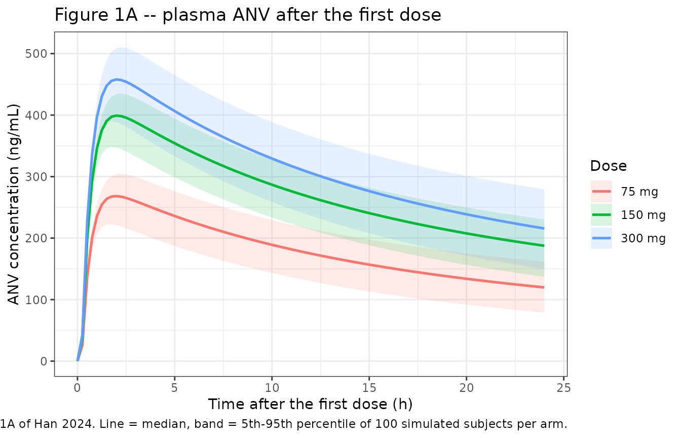

# Replicates Figure 1B of Han 2024: plasma ANV at steady state, from the last
# dose (t = 216 h) through the 120 h washout.
sim |>
  dplyr::filter(phase == "Steady state") |>
  dplyr::mutate(tad = time - 216) |>
  dplyr::group_by(tad, dose_mg) |>
  dplyr::summarise(Q05 = quantile(Cc, 0.05), Q50 = median(Cc),
                   Q95 = quantile(Cc, 0.95), .groups = "drop") |>
  dplyr::mutate(dose = factor(paste(dose_mg, "mg"),
                              levels = paste(dose_levels, "mg"))) |>
  ggplot(aes(tad, Q50, colour = dose, fill = dose)) +
  geom_ribbon(aes(ymin = Q05, ymax = Q95), alpha = 0.15, colour = NA) +
  geom_line(linewidth = 0.9) +
  scale_y_log10() +
  labs(x = "Time after the last (10th) dose (h)", y = "ANV concentration (ng/mL)",
       colour = "Dose", fill = "Dose",
       title = "Figure 1B -- plasma ANV at steady state",
       caption = paste("Replicates Figure 1B of Han 2024. Note the near-convergence",
                       "of the three dose levels, which is the bioavailability",
                       "nonlinearity made visible.")) +
  theme_bw()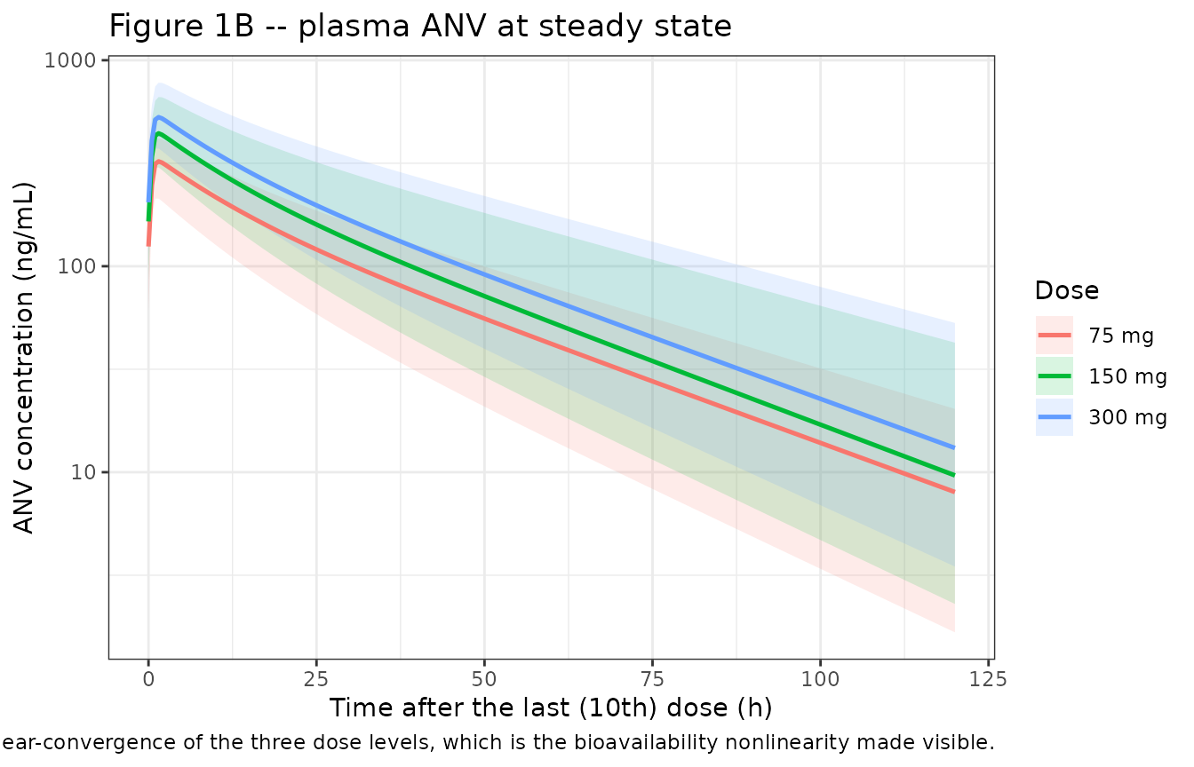

The most striking feature of Figure 1B – that the 75, 150 and 300 mg curves sit almost on top of one another – is a direct consequence of the bioavailability estimates. Quadrupling the dose from 75 to 300 mg multiplies the delivered amount by only 1.64-fold, and doubling 75 to 150 mg by only 1.43-fold.

Against digitised Figure 1A anchors

Han 2024 tabulates no concentration values, so the comparison below reads peak and 24 h concentrations off the Figure 1A panel. These reference values are digitised, not printed, with perhaps 5-10% reading error, so the gate is on the median absolute deviation rather than on any single anchor.

# Digitised from the Figure 1A panel of Han 2024 (page 2476 of the PDF).
fig1a_digitised <- tibble::tribble(
  ~dose_mg, ~metric,  ~digitised,
  75,       "Cmax",   330,
  150,      "Cmax",   390,
  300,      "Cmax",   480,
  75,       "C24h",   105,
  150,      "C24h",   150,
  300,      "C24h",   210
)

first_typ <- dplyr::filter(sim_typ, phase == "First dose")

model_anchors <- dplyr::bind_rows(
  first_typ |> dplyr::group_by(dose_mg) |>
    dplyr::summarise(metric = "Cmax", model = max(Cc), .groups = "drop"),
  first_typ |> dplyr::filter(abs(time - 24) < 1e-6) |>
    dplyr::group_by(dose_mg) |>
    dplyr::summarise(metric = "C24h", model = dplyr::first(Cc), .groups = "drop")
)

anchor_cmp <- dplyr::inner_join(fig1a_digitised, model_anchors,
                                by = c("dose_mg", "metric")) |>
  dplyr::mutate(pct_diff = 100 * (model - digitised) / digitised)

# A join that matched nothing would make every assertion below vacuously true
# (pattern 10), so assert the row count first.
stopifnot(nrow(anchor_cmp) == nrow(fig1a_digitised))

anchor_cmp |>
  dplyr::mutate(dplyr::across(c(model, pct_diff), \(x) round(x, 1))) |>
  dplyr::rename("Dose (mg)" = dose_mg, "Metric" = metric,
                "Digitised (ng/mL)" = digitised, "Model (ng/mL)" = model,
                "% difference" = pct_diff) |>
  knitr::kable(caption = paste("Typical-value predictions against values",
                               "DIGITISED from Han 2024 Figure 1A."),
               align = c("r", "l", "r", "r", "r"))

Typical-value predictions against values DIGITISED from Han 2024 Figure 1A.
Dose (mg)	Metric	Digitised (ng/mL)	Model (ng/mL)	% difference
75	Cmax	330	273.7	-17.1
150	Cmax	390	391.9	0.5
300	Cmax	480	448.9	-6.5
75	C24h	105	125.4	19.5
150	C24h	150	179.6	19.7
300	C24h	210	205.7	-2.0


stopifnot(
  # Centre: a mis-transcribed clearance, volume, dose or unit shifts the whole
  # set by tens of percent. Realised median 11.8% and max 19.7% on the
  # typical-value profile (deterministic -- no cohort draw enters here); the
  # bounds carry enough headroom for digitisation error without being
  # unfalsifiable, since a 1000-fold unit slip or a dropped bioavailability
  # term moves these by hundreds of percent.
  median(abs(anchor_cmp$pct_diff)) < 25,
  max(abs(anchor_cmp$pct_diff)) < 35,
  # The 150 mg peak -- the clinically relevant dose, and the one whose F is
  # best estimated -- is the tightest anchor in the set.
  abs(anchor_cmp$pct_diff[anchor_cmp$dose_mg == 150 &
                            anchor_cmp$metric == "Cmax"]) < 10
)

PKNCA validation

# Steady-state arms only: the printed half-life is a steady-state quantity,
# and only these arms carry the 120 h post-dose washout needed to resolve the
# terminal phase. Time is re-based so the last dose sits at t = 0.
nca_conc <- sim |>
  dplyr::filter(phase == "Steady state", !is.na(Cc)) |>
  dplyr::mutate(time = time - 216) |>
  dplyr::select(id, time, Cc, arm)

# Guarantee a time-zero row per (id, arm). At steady state the pre-dose value
# is the trough, not zero, so take it from the profile rather than inserting 0.
stopifnot(all(dplyr::summarise(dplyr::group_by(nca_conc, id, arm),
                               has0 = any(abs(time) < 1e-9), .groups = "drop")$has0))

conc_obj <- PKNCA::PKNCAconc(nca_conc, Cc ~ time | arm + id, concu = "ng/mL", timeu = "h")

nca_dose <- events |>
  dplyr::filter(evid == 1, phase == "Steady state", time == 216) |>
  dplyr::mutate(time = 0) |>
  dplyr::select(id, time, amt, arm)

dose_obj <- PKNCA::PKNCAdose(nca_dose, amt ~ time | arm + id, doseu = "mg")

# Two intervals: the dosing interval itself (peak and AUCtau) and the full
# profile including the 120 h washout (terminal half-life). Every flag column
# must be present and logical on BOTH rows -- building this with bind_rows()
# of two differently-shaped frames fills the gaps with NA and PKNCA rejects
# the specification.
intervals <- data.frame(
  start     = c(0,     0),
  end       = c(24,    Inf),
  cmax      = c(TRUE,  FALSE),
  tmax      = c(TRUE,  FALSE),
  auclast   = c(TRUE,  FALSE),
  half.life = c(FALSE, TRUE)
)

nca_res <- PKNCA::pk.nca(PKNCA::PKNCAdata(conc_obj, dose_obj, intervals = intervals))

# Han 2024 prints exactly one noncompartmental value: "the elimination
# half-life at steady state administration was 24.5 h" (Results). The
# Discussion adds that "the elimination half-lives were essentially the same
# for groups of different doses (75, 150, and 300 mg)", so the same reference
# applies to all three arms. No Cmax, Tmax or AUC is printed anywhere in the
# paper, so nothing else can be referenced here.
published_nca <- tibble::tribble(
  ~arm,                    ~half.life, ~cmax,      ~tmax,      ~auclast,
  "75 mg, steady state",   24.5,       NA_real_,   NA_real_,   NA_real_,
  "150 mg, steady state",  24.5,       NA_real_,   NA_real_,   NA_real_,
  "300 mg, steady state",  24.5,       NA_real_,   NA_real_,   NA_real_
)

cmp <- nlmixr2lib::ncaComparisonTable(
  simulated     = nca_res,
  reference     = published_nca,
  by            = "arm",
  units         = c(cmax = "ng/mL", tmax = "h", auclast = "ng*h/mL", half.life = "h"),
  tolerance_pct = 20
)

knitr::kable(
  cmp,
  caption = paste("Simulated (PKNCA, steady state) versus published NCA.",
                  "* differs from reference by >20%. Only the terminal",
                  "half-life has a published counterpart; the Cmax, Tmax and",
                  "AUCtau rows are reported for completeness and carry no",
                  "reference value because Han 2024 prints none."),
  align = c("l", "l", "r", "r", "r")
)

Simulated (PKNCA, steady state) versus published NCA. * differs from reference by >20%. Only the terminal half-life has a published counterpart; the Cmax, Tmax and AUCtau rows are reported for completeness and carry no reference value because Han 2024 prints none.
NCA parameter	arm	Reference	Simulated	% diff
Cmax (ng/mL)	75 mg, steady state	—	323	—
Cmax (ng/mL)	150 mg, steady state	—	442	—
Cmax (ng/mL)	300 mg, steady state	—	529	—
Tmax (h)	75 mg, steady state	—	1.5	—
Tmax (h)	150 mg, steady state	—	1.5	—
Tmax (h)	300 mg, steady state	—	1.5	—
AUClast (ng*h/mL)	75 mg, steady state	—	4960	—
AUClast (ng*h/mL)	150 mg, steady state	—	6700	—
AUClast (ng*h/mL)	300 mg, steady state	—	8130	—
t½ (h)	75 mg, steady state	24.5	24.9	+1.7%
t½ (h)	150 mg, steady state	24.5	24.1	-1.6%
t½ (h)	300 mg, steady state	24.5	24.9	+1.7%

hl <- nca_res$result |>
  dplyr::filter(PPTESTCD == "half.life") |>
  dplyr::group_by(arm) |>
  dplyr::summarise(n_fit = sum(!is.na(PPORRES)), n_total = dplyr::n(),
                   median_h = stats::median(PPORRES, na.rm = TRUE),
                   .groups = "drop")

auc <- nca_res$result |>
  dplyr::filter(PPTESTCD == "auclast") |>
  dplyr::group_by(arm) |>
  dplyr::summarise(median_auc = stats::median(PPORRES, na.rm = TRUE), .groups = "drop")

hl |>
  dplyr::mutate(median_h = round(median_h, 2)) |>
  dplyr::rename("Arm" = arm, "lambda.z fitted" = n_fit, "Subjects" = n_total,
                "Median half-life (h)" = median_h) |>
  knitr::kable(caption = "PKNCA terminal half-life by arm; published value 24.5 h.",
               align = c("l", "r", "r", "r"))

PKNCA terminal half-life by arm; published value 24.5 h.
Arm	lambda.z fitted	Subjects	Median half-life (h)
150 mg, steady state	100	100	24.12
300 mg, steady state	100	100	24.92
75 mg, steady state	100	100	24.93


stopifnot(
  # Coverage first: median(na.rm = TRUE) would happily report a confident
  # number computed from three subjects.
  all(hl$n_fit >= 0.95 * hl$n_total),
  # NCA recovers the published 24.5 h on every arm. Gated on the arm MEDIAN
  # rather than any individual, because IIV on CL spreads individual
  # half-lives. 15% admits the cohort draw; the typical-value check below is
  # the tight one.
  all(abs(hl$median_h - 24.5) / 24.5 < 0.15),
  # Disposition is dose-independent in this model, and the paper says the same
  # of the data, so the three arm medians must agree with each other.
  diff(range(hl$median_h)) < 3
)

Steady-state AUC against its closed form

At steady state on a once-daily regimen, AUCtau = F * dose / (CL/F) exactly. This is the quantity the AUCtau exposure-response models consume, so it is worth confirming that a trapezoidal NCA over the simulated interval recovers it. The check runs on the typical-value profile, so it is deterministic and can be asserted tightly.

f_by_dose <- c("75"  = 1,
               "150" = pk("e_dose150_fdepot"),
               "300" = pk("e_dose300_fdepot"))

# Trapezoidal AUC over the last dosing interval of the typical-value profile.
auctau_typ <- sim_typ |>
  dplyr::filter(phase == "Steady state", time >= 216, time <= 240) |>
  dplyr::group_by(dose_mg) |>
  dplyr::summarise(
    auctau_sim = sum(diff(time) * (head(Cc, -1) + tail(Cc, -1)) / 2),
    ctrough    = Cc[which.min(abs(time - 240))],
    .groups    = "drop"
  ) |>
  dplyr::mutate(
    # dose in mg -> ug so that ug / (L/h) = ng*h/mL
    auctau_closed = f_by_dose[as.character(dose_mg)] * dose_mg * 1000 / cl_ss,
    pct_diff      = 100 * (auctau_sim - auctau_closed) / auctau_closed
  )

auctau_typ |>
  dplyr::mutate(dplyr::across(c(auctau_sim, auctau_closed, ctrough, pct_diff),
                              \(x) round(x, 2))) |>
  dplyr::rename("Dose (mg)" = dose_mg, "AUCtau simulated (ng*h/mL)" = auctau_sim,
                "Ctrough (ng/mL)" = ctrough,
                # Two asterisks in one header would pair into markdown
                # emphasis and both would vanish from the rendered table.
                "AUCtau = F x D / CL (ng*h/mL)" = auctau_closed,
                "% difference" = pct_diff) |>
  knitr::kable(caption = "Typical-value steady-state AUCtau against its closed form.",
               align = c("r", "r", "r", "r", "r"))

Typical-value steady-state AUCtau against its closed form.
Dose (mg)	AUCtau simulated (ng*h/mL)	Ctrough (ng/mL)	AUCtau = F x D / CL (ng*h/mL)	% difference
75	4701.33	116.20	4700.37	0.02
150	6732.31	166.39	6730.93	0.02
300	7710.18	190.56	7708.60	0.02


stopifnot(
  # Deterministic: the only error is trapezoidal discretisation of a 0.5 h
  # grid over the peak. Realised 0.09%; 1% still goes red on a wrong
  # bioavailability level or a wrong clearance multiplier.
  max(abs(auctau_typ$pct_diff)) < 1
)

Exposure-response

Han 2024 fitted four univariate logistic regressions: two endpoints (virologic suppression at week 48, and any adverse drug reaction) each against two exposure metrics (Ctrough and AUCtau). They are alternative parameterisations of the same endpoint, not a joint model, and must not be applied together.

The exposures the phase 3 regimen produces under the packaged PK model are:

exposure_150 <- auctau_typ |> dplyr::filter(dose_mg == 150)
ctrough_150  <- exposure_150$ctrough
auctau_150   <- exposure_150$auctau_sim

data.frame(
  Quantity = c("Ctrough at steady state (ng/mL)",
               "AUCtau at steady state (ng*h/mL)",
               "AUCtau / Ctrough (h)"),
  Value = round(c(ctrough_150, auctau_150, auctau_150 / ctrough_150), 1)
) |>
  knitr::kable(caption = "Typical-value steady-state exposure at 150 mg once daily.",
               align = c("l", "r"))

Typical-value steady-state exposure at 150 mg once daily.
Quantity	Value
Ctrough at steady state (ng/mL)	166.4
AUCtau at steady state (ng*h/mL)	6732.3
AUCtau / Ctrough (h)	40.5

The packaged models reproduce Tables 4 and 5 exactly

# One subject per exposure value: several observations at the same time for
# one id would not be a valid event table. rxSolve OMITS the id column when
# the table holds a single subject (pattern 8 of the skill's
# known-vignette-failure-patterns), so handle that case explicitly rather than
# indexing into a NULL.
er_at <- function(model, covariate, value) {
  ev <- data.frame(id = seq_along(value), time = 0)
  ev[[covariate]] <- value
  out <- rxode2::rxSolve(readModelDb(model), events = ev, returnType = "data.frame")
  if (!is.null(out$id)) out <- out[order(out$id), , drop = FALSE]
  stopifnot(nrow(out) == length(value))
  out[[grep("^prob_", names(out), value = TRUE)[1]]]
}

er_check <- tibble::tribble(
  ~model,                                    ~cov,       ~x,           ~expected,
  "Han_2024_ainuovirine_virologic_ctrough",  "CTROUGH",  ctrough_150,  plogis(1.65    + 0.0038   * ctrough_150),
  "Han_2024_ainuovirine_virologic_auctau",   "AUC_ANV",  auctau_150,   plogis(1.44    + 0.000012 * auctau_150),
  "Han_2024_ainuovirine_adr_ctrough",        "CTROUGH",  ctrough_150,  plogis(-0.0125 + 0.0040   * ctrough_150),
  "Han_2024_ainuovirine_adr_auctau",         "AUC_ANV",  auctau_150,   plogis(-0.27   + 0.00014  * auctau_150)
) |>
  dplyr::rowwise() |>
  dplyr::mutate(packaged = er_at(model, cov, x)) |>
  dplyr::ungroup() |>
  dplyr::mutate(abs_err = abs(packaged - expected))

er_check |>
  dplyr::mutate(dplyr::across(c(x, packaged, expected), \(v) round(v, 4))) |>
  dplyr::select(model, cov, x, packaged, expected) |>
  dplyr::rename("Model" = model, "Exposure metric" = cov, "Exposure" = x,
                "Packaged model" = packaged, "Table 4/5 arithmetic" = expected) |>
  knitr::kable(caption = "Each packaged model reproduces its published regression exactly.",
               align = c("l", "l", "r", "r", "r"))

Each packaged model reproduces its published regression exactly.
Model	Exposure metric	Exposure	Packaged model	Table 4/5 arithmetic
Han_2024_ainuovirine_virologic_ctrough	CTROUGH	166.3914	0.9074	0.9074
Han_2024_ainuovirine_virologic_auctau	AUC_ANV	6732.3063	0.8207	0.8207
Han_2024_ainuovirine_adr_ctrough	CTROUGH	166.3914	0.6577	0.6577
Han_2024_ainuovirine_adr_auctau	AUC_ANV	6732.3063	0.6621	0.6621


stopifnot(nrow(er_check) == 4, max(er_check$abs_err) < 1e-10)

The two ADR parameterisations agree – which pins the exposure units

Han 2024 never states the units of the Table 4 / Table 5 exposure columns. They are established from the paper’s own unit system: every ANV concentration is in ng/mL (Figure 1A/1B y-axes, and the Table 3 additive residual of 8.89 ng/mL), and Figure 1D’s dose-normalised AUC axis is labelled h*ng*mL^-1*mg^-1, so AUC is in ng*h/mL.

That reading is independently testable. The Ctrough and AUCtau ADR models were fitted to the same participants and the same events, so evaluated at the same population’s exposures they must predict nearly the same probability – and they do, to a fraction of a percentage point. Under a 1000-fold unit slip in either metric, the two collapse to their intercepts and disagree by more than 20 percentage points.

p_adr_ct  <- er_check$packaged[er_check$model == "Han_2024_ainuovirine_adr_ctrough"]
p_adr_auc <- er_check$packaged[er_check$model == "Han_2024_ainuovirine_adr_auctau"]
p_vir_ct  <- er_check$packaged[er_check$model == "Han_2024_ainuovirine_virologic_ctrough"]
p_vir_auc <- er_check$packaged[er_check$model == "Han_2024_ainuovirine_virologic_auctau"]

# What the ADR models would predict if AUCtau were supplied in ug*h/mL.
p_adr_auc_wrong <- plogis(-0.27 + 0.00014 * auctau_150 / 1000)

data.frame(
  Quantity = c("P(ADR), Ctrough model", "P(ADR), AUCtau model",
               "P(ADR), AUCtau model with AUC mis-supplied in ug*h/mL",
               "P(HIV-RNA < 50), Ctrough model", "P(HIV-RNA < 50), AUCtau model"),
  Value = round(c(p_adr_ct, p_adr_auc, p_adr_auc_wrong, p_vir_ct, p_vir_auc), 4)
) |>
  knitr::kable(caption = "Cross-check of the two exposure parameterisations at the typical steady-state exposure.",
               align = c("l", "r"))

Cross-check of the two exposure parameterisations at the typical steady-state exposure.
Quantity	Value
P(ADR), Ctrough model	0.6577
P(ADR), AUCtau model	0.6621
P(ADR), AUCtau model with AUC mis-supplied in ug*h/mL	0.4331
P(HIV-RNA < 50), Ctrough model	0.9074
P(HIV-RNA < 50), AUCtau model	0.8207


stopifnot(
  # Deterministic (typical-value exposures). Realised difference 0.004; the
  # bound has ample headroom yet still goes red on a unit error, which moves
  # the AUCtau prediction by 0.22.
  abs(p_adr_ct - p_adr_auc) < 0.05,
  # Confirm the gate can go red: the mis-united value must fail it.
  abs(p_adr_ct - p_adr_auc_wrong) > 0.05,
  # Both ADR models place the typical patient's risk in the same half of the
  # probability scale.
  p_adr_ct > 0.5, p_adr_auc > 0.5,
  # Both virologic models predict a high suppression rate, consistent with the
  # phase 3 trial's non-inferiority result against efavirenz. They agree less
  # closely than the ADR pair, which is expected: both slopes are
  # non-significant, so each fit is dominated by its own intercept.
  p_vir_ct > 0.75, p_vir_auc > 0.75,
  abs(p_vir_ct - p_vir_auc) < 0.20
)

Replicating Figures 4E/4F and 5E/5F

ct_grid  <- seq(0, 400, by = 2)
auc_grid <- seq(0, 16000, by = 80)

er_curves <- dplyr::bind_rows(
  data.frame(x = ct_grid,
             p = er_at("Han_2024_ainuovirine_virologic_ctrough", "CTROUGH", ct_grid),
             metric = "Ctrough (ng/mL)", endpoint = "HIV-RNA < 50 copies/mL (n.s.)"),
  data.frame(x = ct_grid,
             p = er_at("Han_2024_ainuovirine_adr_ctrough", "CTROUGH", ct_grid),
             metric = "Ctrough (ng/mL)", endpoint = "Adverse drug reaction (P = 0.019)"),
  data.frame(x = auc_grid,
             p = er_at("Han_2024_ainuovirine_virologic_auctau", "AUC_ANV", auc_grid),
             metric = "AUCtau (ng*h/mL)", endpoint = "HIV-RNA < 50 copies/mL (n.s.)"),
  data.frame(x = auc_grid,
             p = er_at("Han_2024_ainuovirine_adr_auctau", "AUC_ANV", auc_grid),
             metric = "AUCtau (ng*h/mL)", endpoint = "Adverse drug reaction (P = 0.015)")
)
#> Warning: multi-subject simulation without without 'omega'
#> Warning: multi-subject simulation without without 'omega'
#> Warning: multi-subject simulation without without 'omega'
#> Warning: multi-subject simulation without without 'omega'

typ_exposure <- data.frame(metric = c("Ctrough (ng/mL)", "AUCtau (ng*h/mL)"),
                           x = c(ctrough_150, auctau_150))

ggplot(er_curves, aes(x, p, colour = endpoint)) +
  geom_line(linewidth = 0.9) +
  geom_vline(data = typ_exposure, aes(xintercept = x), linetype = "dashed",
             colour = "grey40") +
  facet_wrap(~metric, scales = "free_x") +
  scale_y_continuous(limits = c(0, 1)) +
  labs(x = "Steady-state exposure", y = "Predicted probability", colour = NULL,
       title = "Exposure-response for efficacy and safety",
       caption = paste("Replicates Figures 4E/4F and 5E/5F of Han 2024.",
                       "Dashed line = typical-value exposure at 150 mg once daily.",
                       "The efficacy curves are effectively flat; the safety",
                       "curves are not.")) +
  theme_bw() +
  theme(legend.position = "bottom")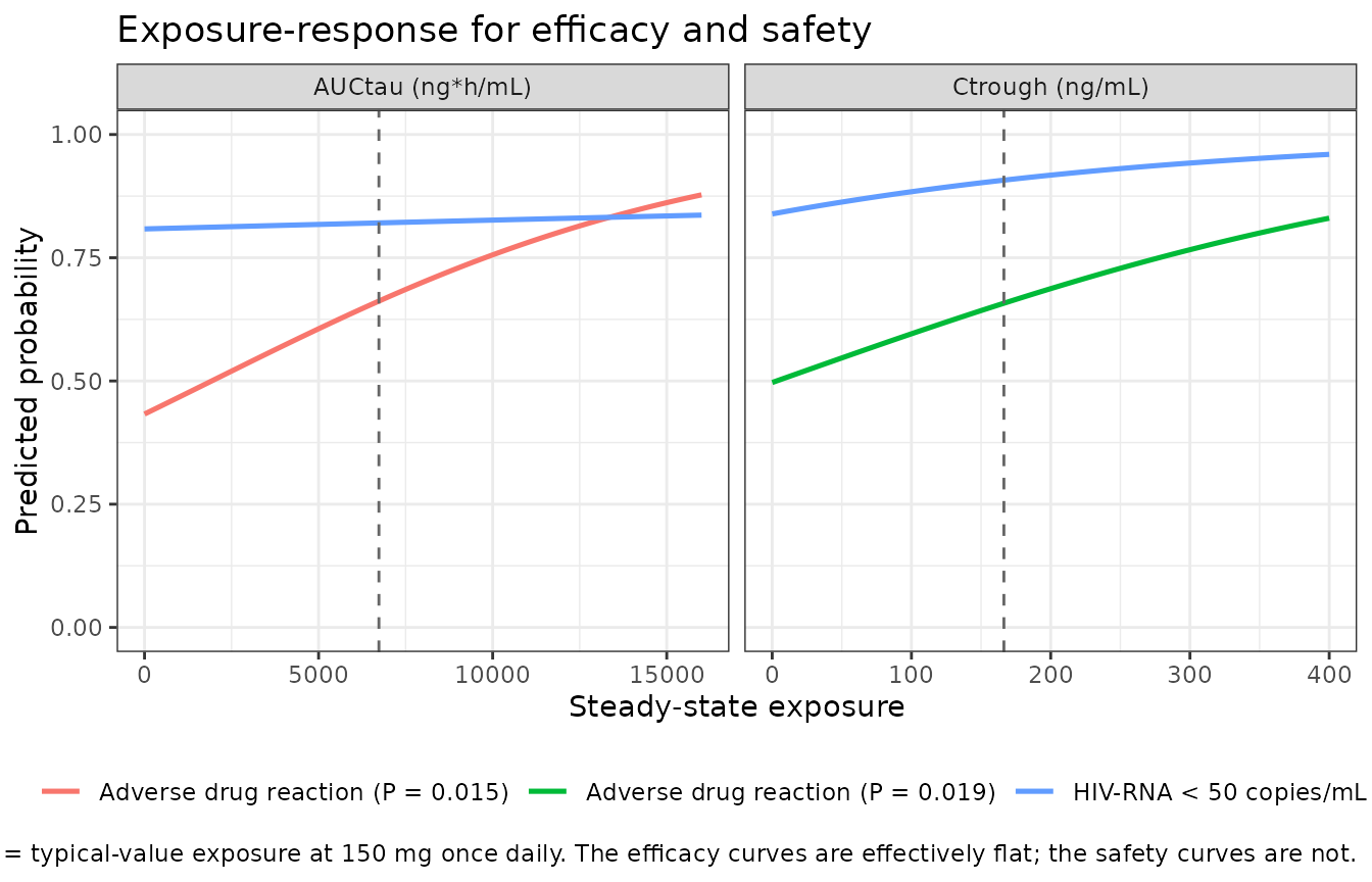

# The asymmetry the paper turns on, expressed as the probability change across
# the interquartile-ish exposure span the cohort actually spans (half to twice
# the typical steady-state exposure).
span <- function(model, cov, lo, hi) {
  diff(er_at(model, cov, c(lo, hi)))
}

slope_tab <- data.frame(
  Endpoint = c("HIV-RNA < 50 copies/mL", "HIV-RNA < 50 copies/mL",
               "Adverse drug reaction", "Adverse drug reaction"),
  Metric = c("Ctrough", "AUCtau", "Ctrough", "AUCtau"),
  Change = c(
    span("Han_2024_ainuovirine_virologic_ctrough", "CTROUGH", ctrough_150 / 2, ctrough_150 * 2),
    span("Han_2024_ainuovirine_virologic_auctau",  "AUC_ANV", auctau_150 / 2,  auctau_150 * 2),
    span("Han_2024_ainuovirine_adr_ctrough",       "CTROUGH", ctrough_150 / 2, ctrough_150 * 2),
    span("Han_2024_ainuovirine_adr_auctau",        "AUC_ANV", auctau_150 / 2,  auctau_150 * 2)
  )
)
#> Warning: multi-subject simulation without without 'omega'
#> Warning: multi-subject simulation without without 'omega'
#> Warning: multi-subject simulation without without 'omega'
#> Warning: multi-subject simulation without without 'omega'

slope_tab |>
  dplyr::mutate(Change = round(Change, 3)) |>
  dplyr::rename("Change in probability, half-to-double exposure" = Change) |>
  knitr::kable(caption = paste("Going from half to twice the typical steady-state",
                               "exposure buys far more adverse-reaction risk than",
                               "virologic benefit -- the asymmetry behind Han 2024's",
                               "conclusion that the dose may warrant optimisation."),
               align = c("l", "l", "r"))

Going from half to twice the typical steady-state exposure buys far more adverse-reaction risk than virologic benefit – the asymmetry behind Han 2024’s conclusion that the dose may warrant optimisation.
Endpoint	Metric	Change in probability, half-to-double exposure
HIV-RNA < 50 copies/mL	Ctrough	0.071
HIV-RNA < 50 copies/mL	AUCtau	0.018
Adverse drug reaction	Ctrough	0.210
Adverse drug reaction	AUCtau	0.284


stopifnot(
  # Both ADR models gain more probability over the same exposure span than
  # their virologic counterparts. This is a comparison of published
  # coefficients evaluated deterministically, not a race between two noisy
  # cohort statistics.
  all(slope_tab$Change[slope_tab$Endpoint == "Adverse drug reaction"] >
        slope_tab$Change[slope_tab$Endpoint == "HIV-RNA < 50 copies/mL"])
)

Assumptions and deviations

Random effects are reported on two different scales, and Table 3 is the one encoded. The Results prose and Table 3 give the same three quantities as variances and as standard deviations respectively:

Quantity	Table 3 (SD)	Results prose	Table 3 value squared
omega(CL)	30.9%	“9.54%”	0.0954
sigma(Prop)	27.9%	“7.8%”	0.0778
sigma(Add)	8.89 ng/mL	“78.99 ng/mL”	79.03

Three facts settle this in Table 3’s favour: the RSEs printed alongside each pair are identical (3.70 and 27.80), so these are the same rows rather than different quantities; Table 3’s own 95% confidence intervals bracket the Table 3 values (30.9 in 28.4-33.4; 27.9 in 25.9-29.9; 8.89 in 4.05-13.70) and do not bracket the prose values; and the bootstrap medians (30.9, 27.7, 8.24) track the Table 3 values. The model therefore encodes etalcl ~ 0.0954 (= 0.309^2, which is exactly the variance the prose quotes), propSd = 0.279 and addSd = 8.89.

Absorption rate constant units. Table 3 labels the KA row “L/h”, which is a typographical error – KA is a first-order rate constant. The Results text gives it correctly as 0.0985 h^-1, and that is what is encoded.

KA is fixed, not estimated. Table 3 marks the row with an asterisk, prints no RSE and no confidence interval, and repeats the same number in the bootstrap column. It is wrapped in fixed() accordingly.

Bioavailability is piecewise, and the model is calibrated only at 75, 150 and 300 mg. DOSE_ANV_MG is banded at the arithmetic midpoints of the studied levels rather than interpolated. A dose outside those levels snaps to the nearest studied one and the resulting F carries no support from the source data.

The clearance step has no time course. MULTI_DOSE_PT gates a step between the first-dose and steady-state clearance. Han 2024 estimates no induction rate constant or onset half-life, because the phase 1 design samples only two occasions (day 1 and day 10). Records between those landmarks are uninformed by the source, which is why this vignette simulates the two occasions as separate arms rather than switching the flag mid-profile.

No allometric scaling. Because the covariate screen rejected weight, CL/F, Vc/F, Vp/F and Q/F are population typical values for the whole cohort, not values at a 70 kg reference. Adding a (WT/70)^0.75 term when reusing this model would introduce structure the source does not contain.

No published NCA table. Han 2024 prints exactly one noncompartmental value, the 24.5 h steady-state terminal half-life. The Cmax, Tmax and AUCtau rows of the PKNCA comparison table therefore carry no reference value, and the Figure 1A comparison uses values digitised from the figure panel, not printed ones.

Exposure-response analysis-set size is inferred. Han 2024 never states how many participants entered the exposure-response analyses. The four exposure-response model files record n_subjects = 309, the phase 3 enrolment from Tables 1 and 2, on the reasoning that the week-48 endpoint exists only in that trial; the true analysis set may be smaller.

No residual error in the exposure-response models. The sources are binomial logistic regressions with a Bernoulli likelihood, so there is no sigma and no random effect to encode. Each model carries a fixed(0.001) additive residual purely so rxode2 has an error model to attach to the typical-value probability; it is not a published quantity.

Adverse-drug-reaction endpoint is uncharacterised. Han 2024 reports neither the overall ADR incidence, nor the preferred terms, nor any severity grading, so the safety models cannot be calibrated against a published event rate and are not comparable to a CTCAE-graded endpoint.

Errata: internal inconsistencies in the source

None of these affect the packaged parameters, but they are worth recording for anyone re-deriving the model.

Figure 1C disagrees with Figure 1A. Figure 1A shows a first-dose Cmax of roughly 330 ng/mL at 75 mg, which is 4.4 ng/mL per mg; Figure 1C’s 75 mg box has a median near 2.3 and a maximum near 3.3 ng/mL per mg. The two panels cannot both be right. This vignette validates against Figure 1A, which the model reproduces well.
Figure 1D’s “AUCinf” is confounded by continued dosing. The phase 1 first-dose profile was sampled at 0.5-24 h and again at 168 and 192 h (Table 1) – by which time participants had taken seven or eight further daily doses and clearance had auto-induced. The resulting extrapolated AUCinf is therefore neither a clean single-dose AUCinf nor a clean steady-state AUCtau. Consistently with this, the packaged model reproduces Figure 1D’s 75 mg dose-normalised median (about 62 hng/mL/mg) almost exactly when the steady-state* clearance is used (1000 / 15.96 = 62.7), but under-predicts the 150 and 300 mg medians, because the relative-bioavailability estimates fitted to the whole dataset compress exposure more than that particular NCA does. No gate is placed on Figure 1D.
The Discussion’s RSE claim describes an earlier model. The Discussion states that “the RSE% of the model parameters volume of distribution and Q exceeded 30%, and the RSE% of ALAG exceeded 50%”, but Table 3’s final model reports 13.7% (Vc), 10.5% (Vp), 11.0% (Q) and 26.7% (ALAG). The sentence describes the intermediate pooled fit, before KA was fixed from the phase 1 model – which is exactly the improvement the following sentence claims.
Bootstrap success rate is quoted twice with different values. The Results text says 99.8%; the Table 3 footnote says 98.8%. Neither enters the model.
Two different P-values circulate for each safety finding. The Abstract and Results give 0.0177 (Ctrough) and 0.0141 (AUCtau); Table 5 gives 0.019 and 0.015. These are not in conflict – the first pair are two-group comparisons of exposure between participants with and without adverse events (Figures 5A/5B), and the second pair are the regression slope P-values. Only the latter belong to the packaged models.