Lumefantrine PK and 28-day recurrence (Tchaparian 2016)
Source:vignettes/articles/Tchaparian_2016_lumefantrine.Rmd
Tchaparian_2016_lumefantrine.RmdModel and source
Tchaparian 2016 reports two models, extracted here as two files and validated in this single vignette.
Tchaparian_2016_lumefantrine– the two-compartment population PK model (Table 2).Tchaparian_2016_lumefantrine_recurrence– the adjusted Cox proportional-hazards model for 28-day recurrent parasitaemia (Table 3), plus the paper’s comparative day-3-versus-day-7 exposure analysis.Citation: Tchaparian E, Sambol NC, Arinaitwe E, McCormack SA, Bigira V, Wanzira H, Muhindo M, Creek DJ, Sukumar N, Blessborn D, Tappero JW, Kakuru A, Bergqvist Y, Aweeka FT, Parikh S. Population pharmacokinetics and pharmacodynamics of lumefantrine in young Ugandan children treated with artemether-lumefantrine for uncomplicated malaria. J Infect Dis. 2016;214(8):1243-1251. doi:10.1093/infdis/jiw338. Parameter values are from Table 2; the covariate model for F is the display equation in Results, ‘Population Pharmacokinetic Model’; the statement that the Q/F and V2/F variances were constrained to 50 percent CV is in the Supplement, ‘Population Pharmacokinetic analysis’.
Article: J Infect Dis. 2016;214(8):1243-1251
Open-access record: PMC5034953
Supplement: published with the open-access article, PMC5034953 (
supp_jiw338_jiw338supp.docx). It is load-bearing for this extraction – see “The supplement settles the omega scale” below.
pk <- rxode2::rxode2(readModelDb("Tchaparian_2016_lumefantrine"))
#> ℹ parameter labels from comments will be replaced by 'label()'
#> Warning: some etas defaulted to non-mu referenced, possible parsing error: etaiov_cl_1, etaiov_cl_2, etaiov_cl_3, etaiov_cl_4, etaiov_cl_5, etaiov_vc_1, etaiov_vc_2, etaiov_vc_3, etaiov_vc_4, etaiov_vc_5, etaiov_q_1, etaiov_q_2, etaiov_q_3, etaiov_q_4, etaiov_q_5, etaiov_vp_1, etaiov_vp_2, etaiov_vp_3, etaiov_vp_4, etaiov_vp_5, etaiov_fdepot_1, etaiov_fdepot_2, etaiov_fdepot_3, etaiov_fdepot_4, etaiov_fdepot_5
#> as a work-around try putting the mu-referenced expression on a simple line
pd <- rxode2::rxode2(readModelDb("Tchaparian_2016_lumefantrine_recurrence"))
The supplement settles the omega scale
Table 2’s variability columns are headed only IIV, % and
IOV (%), which is exactly the ambiguity that ships as a
wrong model. The supplement resolves it in so many words:
“Due to the sparsity of the data, IIV and IOV of Q/F and V2/F were each fixed to be 50% (CV).”
and the Results text corroborates it for clearance (“2.19 L/h, with
8% (CV) interindividual variability”). Both columns are
therefore log-normal CV%, not variances, so every entry
is converted as omega^2 = log(CV^2 + 1). Reading them as
variances instead would have shrunk the coefficient of variation on
bioavailability from 34.9% to 59% on the log scale – a different
model.
The supplement also supplies three further facts used above: that
correlation among CL/F, V1/F, Q/F and V2/F was induced through
variability on F rather than through an estimated covariance block
(which is why this model has no ini() correlation block);
that the residual was combined additive plus proportional; and that the
final model centred weight and age on a one-year-old “for ease of
interpretation”, which is what anchors the Table 2 estimates at 8.43 kg
and 12 months rather than at the cohort median of 9.0 kg.
Population
Two-compartment population PK model with first-order absorption and linear elimination for oral lumefantrine in capillary whole blood of 101 Ugandan children aged 6 months to 2 years (207 malaria episodes, 806 concentrations) treated with artemether-lumefantrine for uncomplicated malaria (Tchaparian 2016). Absorption feeds a depot compartment at a rate constant held at the literature value 0.45 1/h because the study had too few absorption-phase samples to estimate it. Body-weight allometric scaling is applied unconditionally to every disposition parameter (exponent 0.75 shared by CL/F and Q/F, exponent 1 shared by V1/F and V2/F), referenced to 8.43 kg, the typical weight of a 1-year-old child. Age is the single retained covariate and acts on relative bioavailability as the power function F = (AGE_months / 12)^0.596, so a 6-month-old has F = 0.66 and a 2-year-old F = 1.51 relative to the 1-year-old reference - an increase with maturation, which the authors note is the opposite of what CYP3A4 and P-glycoprotein ontogeny would predict and attribute to immature biliary function limiting the dissolution of this highly lipophilic drug in the youngest children. Because every disposition term is apparent (divided by F), correlation among CL/F, V1/F, Q/F and V2/F is induced through variability on F itself rather than through an estimated covariance block. Both interindividual and interoccasion variability are carried on all five parameters, with the occasion being a malaria episode (up to 5 per child); the Q/F and V2/F variances were constrained to 50 percent CV by the authors because the data were too sparse to estimate them. The residual is combined additive plus proportional. The fit was a Monolix 4.3 SAEM run in which the 23 percent of samples below the limit of detection were retained as left-censored.
The PK analysis set is 101 Ugandan children aged 6 months to 2 years, treated for 207 malaria episodes and contributing 806 evaluable capillary whole-blood concentrations; the outcomes analysis set is 100 children over 222 episodes. Baseline characteristics are Table 1. Every child weighed under 14 kg and so received the identical regimen: one artemether-lumefantrine tablet (20 mg artemether plus 120 mg lumefantrine) twice daily for three days, six doses and 720 mg of lumefantrine in total. Morning doses were given in clinic with fat-containing milk to standardise the well-known food effect on lumefantrine absorption; evening doses were given at home.
Two features of the analysis matter for reading everything below.
The matrix is capillary whole blood on filter paper, not
venous plasma. The assay had an LLOQ of 132 ng/mL and an LOD of
52 ng/mL; 188 of 806 samples (23.3%) fell below the LOD and were
retained as left-censored rather than discarded, which is the only
reason the model can describe the 14-day tail at all. The authors devote
a Discussion paragraph to the point that venous plasma runs higher, so
the apparent volumes and exposures here are not directly comparable with
the plasma-based lumefantrine models elsewhere in this library
(Hoglund_2015_lumefantrine,
Kloprogge_2018_lumefantrine,
Ding_2026_lumefantrine).
The recurrence endpoint is dominated by reinfection, not recrudescence. At 63 days, 95.9% of recurrences genotyped as new infection. Tororo district has an entomological inoculation rate up to 562 infective bites per person-year, so the hazard modelled below should be read as post-treatment prophylaxis rather than as a cure rate.
Source trace
Every ini() value and every non-obvious
model() equation, with the place in the source it came
from.
| Parameter | Value | Source |
|---|---|---|
| lcl | log(2.19) L/h | Table 2, CL/F point estimate (RSE 8%); Results repeats ‘CL/F in a typical 12-month-old child is 2.19 L/h’ |
| lvc | log(83.2) L | Table 2, V1/F point estimate per 8.43 kg (RSE 7%) |
| lq | log(0.23) L/h | Table 2, Q/F point estimate (RSE 35%) |
| lvp | log(441) L | Table 2, V2/F point estimate per 8.43 kg (RSE 74%) |
| lka (fixed) | log(0.45) 1/h | Table 2 footnote c; Methods: ka ‘fixed to the previously reported value of 0.45 h-1’ |
| lfdepot (fixed) | log(1) | Table 2 footnote c, F = 1 – the apparent-parameter anchor |
| e_wt_cl_q (fixed) | 0.75 | Table 2 footnote a: ‘Pk * [WT/8.43]^0.75’; Methods imposes it unconditionally |
| e_wt_vc_vp (fixed) | 1 | Methods: volumes multiplied by [weight/reference weight] |
| e_age_fdepot | 0.596 | Table 2 ‘Age effect’ (RSE 38%), footnote b; Results equation F_i = [1 * Age_i/12]^0.596 |
| WT_REF | 8.43 kg | Table 2 footnote a; Supplement: final model centred on a one-year-old |
| AGE_REF_MO | 12 months | Results covariate equation; Table 2 footnote b |
| etalcl | log(0.08^2+1) = 0.00638 | Table 2 CL/F IIV 8% CV (RSE 174) |
| etalvc | log(0.152^2+1) = 0.02284 | Table 2 V1/F IIV 15.2% CV (RSE 46) |
| etalq, etalvp (fixed) | log(0.5^2+1) = 0.22314 | Table 2 footnote c; Supplement: ‘IIV and IOV of Q/F and V2/F were each fixed to be 50% (CV)’ |
| etalfdepot | log(0.349^2+1) = 0.11494 | Table 2 F row, IIV 34.9% CV (RSE 23) |
| etaiov_cl_* | log(0.093^2+1) = 0.00861 | Table 2 CL/F IOV 9.3% (RSE 105) |
| etaiov_vc_* | log(0.086^2+1) = 0.00737 | Table 2 V1/F IOV 8.6% (RSE 133) |
| etaiov_q_, etaiov_vp_ (fixed) | log(0.5^2+1) = 0.22314 | Table 2 footnote c; Supplement as above |
| etaiov_fdepot_* | log(0.594^2+1) = 0.30220 | Table 2 F row, IOV 59.4% (RSE 8) |
| propSd | 0.378 | Table 2 Proportional 37.8% (RSE 5); Results names it a standard deviation |
| addSd | 19.2 ng/mL | Table 2 Additive 19.2 ng/mL (RSE 18) |
| Cc = 1000 * central / vc | unit conversion | Dose in mg and vc in L give mg/L = ug/mL; Table 2 and Figures 1-2 report ng/mL |
| Parameter | Value | Source |
|---|---|---|
| conc_cut (fixed) | 200 ng/mL | Table 3 row heading ‘<200 ng/mL’; Results ROC analysis, area under the curve 0.684 |
| e_conc_lumefantrine_168h_low_haz_nots | log(2.97) | Table 3, ‘Without TMP-SMZ use’ block: adjusted HR 2.97 (1.59-5.55), P = .0007 |
| e_conc_lumefantrine_168h_low_haz_ts | log(0.50) | Table 3, ‘With TMP-SMZ use’ block: adjusted HR 0.50 (0.22-1.13), P = .10 |
| e_conmed_tmpsmx_haz | log(0.75) | Table 3, ‘TMP-SMZ use / Yes’: adjusted HR 0.75 (0.43-1.29), P = .30 |
| age_cut1, age_cut2 (fixed) | 1.0, 1.5 years | Table 3 age strata 6-12, 12-18 and >=18 months |
| e_age_haz_12to18 | log(1.87) | Table 3, age 12-18 mo: adjusted HR 1.87 (0.83-4.22), P = .13 |
| e_age_haz_ge18 | log(1.53) | Table 3, age >=18 mo: adjusted HR 1.53 (0.64-3.63), P = .34 |
| e_residence_rural_haz | log(1.21) | Table 3, ‘Residence / Rural’: adjusted HR 1.21 (0.43-3.43), P = .71 |
| hgb_ref (fixed) | 10.0 g/dL | Table 1 PK-outcomes column, haemoglobin median (centring value; see deviations) |
| e_hgb_haz | log(0.93) | Table 3 haemoglobin, footnote a continuous: adjusted HR 0.93 (0.83-1.05), P = .25 |
| para_ref (fixed) | 17603 parasites/uL | Table 1 PK-outcomes column, geometric mean (centring value; see deviations) |
| e_para_haz | log(1.04) | Table 3 parasite density, footnote a continuous: adjusted HR 1.04 (0.95-1.14), P = .35 |
| waz_cut (fixed) | -2 | Methods: ‘a weight-for-age z score with a -2 cutoff’, WHO standards; Table 3 footnote b |
| e_waz_underweight_haz | log(1.04) | Table 3, ‘Underweight / Yes’: adjusted HR 1.04 (0.47-2.31), P = .93 |
| conc_day3_ref (fixed) | 2777 ng/mL | Results: day 3 median 2777 ng/mL (IQR 1672-4760, n = 187) |
| conc_day7_ref (fixed) | 216 ng/mL | Results: day 7 median 216 ng/mL (IQR 136-345, n = 216) |
| e_conc_lumefantrine_72h_haz | log(0.51) | Results: ‘49% reduced hazard’ per ln unit on day 3, P = .002; Discussion prints 0.51 |
| e_conc_lumefantrine_168h_haz | log(0.80) | Results: ‘20% reduced hazard’ per ln unit on day 7, P = .002; Discussion prints 0.80 |
Structural checks on the PK model
These run on the typical individual with the random effects zeroed, so they are deterministic: no cohort is drawn and the tolerances are numerical rather than statistical.
The ODEs really do integrate the published two-compartment model
The model names its parameters cl / vc /
q / vp, which in rxode2 can trigger the
solved-system path and silently discard an explicitly written
d/dt(). It does not here – but that is worth proving rather
than assuming, so the solve is compared against the closed-form oral
two-compartment biexponential built independently from the same
numbers.
pk0 <- rxode2::zeroRe(pk)
#> Warning: some etas defaulted to non-mu referenced, possible parsing error: etaiov_cl_1, etaiov_cl_2, etaiov_cl_3, etaiov_cl_4, etaiov_cl_5, etaiov_vc_1, etaiov_vc_2, etaiov_vc_3, etaiov_vc_4, etaiov_vc_5, etaiov_q_1, etaiov_q_2, etaiov_q_3, etaiov_q_4, etaiov_q_5, etaiov_vp_1, etaiov_vp_2, etaiov_vp_3, etaiov_vp_4, etaiov_vp_5, etaiov_fdepot_1, etaiov_fdepot_2, etaiov_fdepot_3, etaiov_fdepot_4, etaiov_fdepot_5
#> as a work-around try putting the mu-referenced expression on a simple line
stopifnot(identical(pk$state, c("depot", "central", "peripheral1")))
stopifnot(isFALSE(pk$predDf$linCmt[1]))

wt_med <- 9.1
age_med_mo <- 14.4
dose_mg <- 120

ev1 <- rxode2::et(amt = dose_mg, cmt = "depot", time = 0) |>
  rxode2::et(seq(0, 1000, by = 0.05), cmt = "central")
ev1 <- as.data.frame(ev1)
ev1$WT <- wt_med
ev1$AGE <- age_med_mo / 12
ev1$OCC <- 1

s1 <- rxode2::rxSolve(pk0, ev1, returnType = "data.frame", atol = 1e-12, rtol = 1e-10)
#> ℹ omega/sigma items treated as zero: 'etalcl', 'etalvc', 'etalq', 'etalvp', 'etalfdepot', 'etaiov_cl_1', 'etaiov_cl_2', 'etaiov_cl_3', 'etaiov_cl_4', 'etaiov_cl_5', 'etaiov_vc_1', 'etaiov_vc_2', 'etaiov_vc_3', 'etaiov_vc_4', 'etaiov_vc_5', 'etaiov_q_1', 'etaiov_q_2', 'etaiov_q_3', 'etaiov_q_4', 'etaiov_q_5', 'etaiov_vp_1', 'etaiov_vp_2', 'etaiov_vp_3', 'etaiov_vp_4', 'etaiov_vp_5', 'etaiov_fdepot_1', 'etaiov_fdepot_2', 'etaiov_fdepot_3', 'etaiov_fdepot_4', 'etaiov_fdepot_5'
s1 <- s1[!is.na(s1$Cc) & s1$time > 0, ]

# Independent closed form, built from the Table 2 numbers directly.
cl_i <- 2.19 * (wt_med / 8.43)^0.75
vc_i <- 83.2 * (wt_med / 8.43)
q_i <- 0.23 * (wt_med / 8.43)^0.75
vp_i <- 441 * (wt_med / 8.43)
ka_i <- 0.45
f_i <- (age_med_mo / 12)^0.596
kel_i <- cl_i / vc_i
k12_i <- q_i / vc_i
k21_i <- q_i / vp_i
bsum <- kel_i + k12_i + k21_i
bprod <- kel_i * k21_i
alpha <- (bsum + sqrt(bsum^2 - 4 * bprod)) / 2
beta <- (bsum - sqrt(bsum^2 - 4 * bprod)) / 2
amp <- f_i * dose_mg * ka_i / vc_i
analytic <- 1000 * amp * (
  (k21_i - alpha) / ((ka_i - alpha) * (beta - alpha)) * exp(-alpha * s1$time) +
    (k21_i - beta) / ((ka_i - beta) * (alpha - beta)) * exp(-beta * s1$time) +
    (k21_i - ka_i) / ((alpha - ka_i) * (beta - ka_i)) * exp(-ka_i * s1$time)
)
rel_err <- max(abs(s1$Cc - analytic) / analytic)

# Pure numerical agreement between two exact forms of the same system, so this
# bound is a machine-precision bound and is deliberately tight. Realised
# 1.1e-11; anything above 1e-6 means the ODEs are not the system above.
stopifnot(rel_err < 1e-6)
sprintf("closed-form biexponential agreement: max relative error %.2e over %d points", rel_err, nrow(s1))
#> [1] "closed-form biexponential agreement: max relative error 1.06e-11 over 20000 points"
Dose, clearance, bioavailability and units are mutually consistent
CL/F * AUC(0-inf) = F * Dose must hold exactly for a
linear model with a single input path. This is one gate that
simultaneously exercises the transcribed clearance, the allometric
exponent, the age-on-F power function, the 720 mg course and the ng/mL
unit conversion.
ev2 <- rxode2::et(amt = dose_mg, cmt = "depot", time = seq(0, 60, by = 12)) |>
  rxode2::et(seq(0, 20000, by = 0.5), cmt = "central")
ev2 <- as.data.frame(ev2)
ev2$WT <- wt_med
ev2$AGE <- age_med_mo / 12
ev2$OCC <- 1
s2 <- rxode2::rxSolve(pk0, ev2, returnType = "data.frame", atol = 1e-12, rtol = 1e-10)
#> ℹ omega/sigma items treated as zero: 'etalcl', 'etalvc', 'etalq', 'etalvp', 'etalfdepot', 'etaiov_cl_1', 'etaiov_cl_2', 'etaiov_cl_3', 'etaiov_cl_4', 'etaiov_cl_5', 'etaiov_vc_1', 'etaiov_vc_2', 'etaiov_vc_3', 'etaiov_vc_4', 'etaiov_vc_5', 'etaiov_q_1', 'etaiov_q_2', 'etaiov_q_3', 'etaiov_q_4', 'etaiov_q_5', 'etaiov_vp_1', 'etaiov_vp_2', 'etaiov_vp_3', 'etaiov_vp_4', 'etaiov_vp_5', 'etaiov_fdepot_1', 'etaiov_fdepot_2', 'etaiov_fdepot_3', 'etaiov_fdepot_4', 'etaiov_fdepot_5'
s2 <- s2[!is.na(s2$Cc), ]
auc_numeric <- sum(diff(s2$time) * (head(s2$Cc, -1) + tail(s2$Cc, -1)) / 2) / 1000
auc_identity <- f_i * 6 * dose_mg / cl_i

stopifnot(abs(auc_numeric / auc_identity - 1) < 1e-3)
sprintf(
  "AUC(0-inf): numeric %.2f vs F*Dose/CL %.2f ug*h/mL (relative difference %.1e); published median 347.8",
  auc_numeric, auc_identity, abs(auc_numeric / auc_identity - 1)
)
#> [1] "AUC(0-inf): numeric 345.99 vs F*Dose/CL 346.07 ug*h/mL (relative difference 2.5e-04); published median 347.8"
The age-on-bioavailability function reproduces the Discussion
The Discussion states the model “predicts a point estimate of relative bioavailability of 0.7 for a 6-month-old child as compared to 1.5 in a 2-year-old child, with a value of 1 for the reference 1-year-old population”. Those three numbers are an independent check on the 0.596 exponent and on the 12-month reference age.
f_at <- function(months) (months / 12)^0.596
f_tab <- tibble::tibble(
  `Age` = c("6 months", "12 months (reference)", "24 months"),
  `Model F` = round(f_at(c(6, 12, 24)), 3),
  `Discussion` = c(0.7, 1.0, 1.5)
)
knitr::kable(f_tab, caption = "Relative bioavailability versus age (Tchaparian 2016 Discussion).")| Age | Model F | Discussion |
|---|---|---|
| 6 months | 0.662 | 0.7 |
| 12 months (reference) | 1.000 | 1.0 |
| 24 months | 1.512 | 1.5 |
Time to the limit of detection
Results states that “half of all children are predicted to reach the
LOD (52 ng/mL) in approximately 10 days”. This is the only statement the
paper makes about the shape of the terminal decline, so it is the only
available check on Q/F and V2/F – the two
least precisely estimated parameters in Table 2 (RSE 35% and 74%).
s_lod <- s2[s2$time > 100, ]
t_lod <- s_lod$time[which(s_lod$Cc < 52)[1]] / 24

stopifnot(abs(t_lod - 10) < 1.5)
sprintf("typical child crosses the 52 ng/mL LOD at %.2f days (paper: approximately 10 days)", t_lod)
#> [1] "typical child crosses the 52 ng/mL LOD at 9.56 days (paper: approximately 10 days)"
Virtual cohort
The cohort is calibrated to Tchaparian 2016 Table 1 rather than to an external growth standard, because the model’s two covariates are weight and age and it is the paper’s own marginal distributions that the published exposure summaries are conditioned on. Age is drawn uniformly across the observed range and weight from a weight-for-age line anchored on the cohort median, with log-normal scatter tuned so that the simulated weight median and range match the published ones. This cohort runs visibly lighter than the WHO median for age – the paper reports a median weight-for-age z score of -0.74 – which is the intended behaviour.
Cohort size is 200, the per-arm cap for this repository; a single treatment arm is simulated because every child in the study received the same regimen.
rxode2::rxSetSeed(20260922L)
set.seed(20260922L)
n_sub <- 200L

age_mo <- runif(n_sub, 6.6, 22.2)
wt_kg <- (6.95 + 0.149 * age_mo) * exp(rnorm(n_sub, 0, 0.115))
wt_kg <- pmin(pmax(wt_kg, 6.1), 13.0)

cohort <- tibble::tibble(id = seq_len(n_sub), WT = wt_kg, AGE = age_mo / 12, OCC = 1)

cohort_tab <- tibble::tibble(
  Characteristic = c("Weight, kg", "Age, months"),
  Simulated = c(
    sprintf("%.1f (%.1f-%.1f)", median(wt_kg), min(wt_kg), max(wt_kg)),
    sprintf("%.1f (%.1f-%.1f)", median(age_mo), min(age_mo), max(age_mo))
  ),
  `Table 1` = c("9.1 (6.1-13.0)", "14.4 (6.6-22.2)")
)
knitr::kable(cohort_tab, caption = "Simulated cohort versus Tchaparian 2016 Table 1, median (range).")| Characteristic | Simulated | Table 1 |
|---|---|---|
| Weight, kg | 9.2 (6.5-13.0) | 9.1 (6.1-13.0) |
| Age, months | 14.9 (6.6-22.2) | 14.4 (6.6-22.2) |
# Gate the cohort itself: if the covariate distributions drift, every exposure
# comparison below becomes uninterpretable. Bounds are on the median only --
# the extremes of a random cohort are not reproducible across rxode2 builds.
stopifnot(
  abs(median(wt_kg) / 9.1 - 1) < 0.10,
  abs(median(age_mo) / 14.4 - 1) < 0.10
)
Simulation
Six doses of 120 mg at 0, 12, 24, 36, 48 and 60 h, matching the study’s twice-daily three-day course. The observation grid is log-spaced through the dosing period so that the peak is resolved, then dense to 96 h and coarser out to 1512 h (63 days, the paper’s secondary follow-up horizon).
Note the landmark arithmetic: Methods define day 3 as “12 hours after the last dose” and day 7 as “108 hours after the last dose”. With the last of the six doses at 60 h, the two landmarks are 72 h and 168 h after the first dose.
obs_times <- sort(unique(c(
  exp(seq(log(0.05), log(60), length.out = 60)),
  seq(0, 96, by = 1),
  seq(100, 1512, by = 4)
)))

ev_one <- rxode2::et(amt = dose_mg, cmt = "depot", time = seq(0, 60, by = 12)) |>
  rxode2::et(obs_times, cmt = "central")
ev_one <- as.data.frame(ev_one)

# Covariates must be attached to a materialized data frame: assigning them to
# an rxEt object silently drops them.
events <- do.call(rbind, lapply(seq_len(n_sub), function(i) {
  one <- ev_one
  one$id <- cohort$id[i]
  one$WT <- cohort$WT[i]
  one$AGE <- cohort$AGE[i]
  one$OCC <- cohort$OCC[i]
  one
}))

sim <- rxode2::rxSolve(pk, events, returnType = "data.frame")
obs <- sim |> dplyr::filter(!is.na(Cc))

per_id <- obs |>
  dplyr::group_by(id) |>
  dplyr::summarise(
    cmax = max(Cc),
    tmax = time[which.max(Cc)],
    c72 = Cc[which.min(abs(time - 72))],
    c168 = Cc[which.min(abs(time - 168))],
    cl_i = dplyr::first(cl),
    f_ind = dplyr::first(fdepot),
    .groups = "drop"
  ) |>
  dplyr::mutate(auc_model = f_ind * 6 * dose_mg / cl_i)
Cc is the individual prediction and carries no residual
error, which is the right quantity to compare against the paper’s
model-predicted summaries.
Replicating Figure 2
Figure 2 of Tchaparian 2016 shows the predicted concentration distribution against the observed data, with the median and nested prediction intervals shaded. Below is the same construction from the packaged model, with the assay LOD and LLOQ and the 200 ng/mL efficacy threshold marked.
band <- obs |>
  dplyr::filter(time > 0, time <= 504) |>
  dplyr::group_by(time) |>
  dplyr::summarise(
    lo90 = quantile(Cc, 0.05), lo50 = quantile(Cc, 0.25),
    med = median(Cc),
    hi50 = quantile(Cc, 0.75), hi90 = quantile(Cc, 0.95),
    .groups = "drop"
  )

ggplot(band, aes(x = time / 24)) +
  geom_ribbon(aes(ymin = lo90, ymax = hi90), alpha = 0.18, fill = "steelblue") +
  geom_ribbon(aes(ymin = lo50, ymax = hi50), alpha = 0.35, fill = "steelblue") +
  geom_line(aes(y = med), linewidth = 0.9) +
  geom_hline(yintercept = c(52, 132, 200), linetype = c("dotted", "dotted", "dashed"),
             colour = c("grey40", "grey40", "firebrick")) +
  geom_vline(xintercept = c(3, 7), linetype = "dotdash", colour = "grey55") +
  scale_y_log10() +
  labs(
    x = "Days after the first dose",
    y = "Lumefantrine, capillary whole blood (ng/mL)"
  ) +
  theme_bw()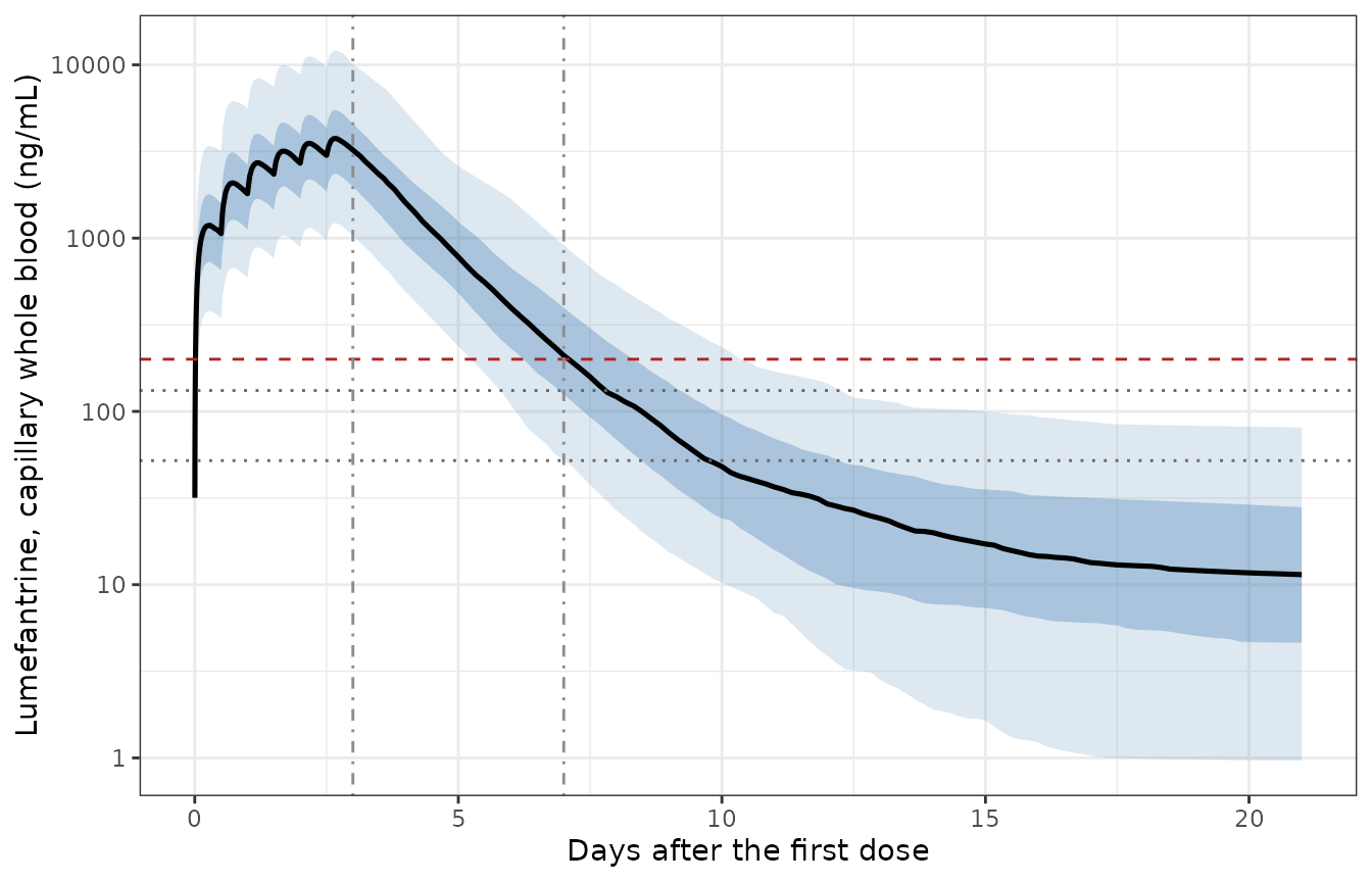
Replicates Figure 2 of Tchaparian 2016: predicted capillary whole-blood lumefantrine concentration versus time, median with 50% and 90% prediction intervals. Horizontal lines mark the assay LOD (52 ng/mL), the LLOQ (132 ng/mL) and the 200 ng/mL day-7 efficacy threshold; vertical lines mark the day 3 and day 7 landmarks.
PKNCA validation
sim_nca <- obs |>
  dplyr::mutate(treatment = "AL 120 mg BID x 3 d") |>
  dplyr::select(id, time, Cc, treatment)

# Guarantee a time-zero record so PKNCA does not warn about an AUC interval
# starting before the first measurement. Pre-dose concentration is 0 for an
# extravascular model.
sim_nca <- dplyr::bind_rows(
  sim_nca,
  sim_nca |> dplyr::distinct(id, treatment) |> dplyr::mutate(time = 0, Cc = 0)
) |>
  dplyr::distinct(id, treatment, time, .keep_all = TRUE) |>
  dplyr::arrange(id, treatment, time)

dose_df <- events |>
  dplyr::filter(evid == 1) |>
  dplyr::mutate(treatment = "AL 120 mg BID x 3 d") |>
  dplyr::select(id, time, amt, treatment)

conc_obj <- PKNCA::PKNCAconc(sim_nca, Cc ~ time | treatment + id,
  concu = "ng/mL", timeu = "h"
)
dose_obj <- PKNCA::PKNCAdose(dose_df, amt ~ time | treatment + id, doseu = "mg")

intervals <- data.frame(
  start = 0, end = Inf,
  cmax = TRUE, tmax = TRUE, auclast = TRUE, aucinf.obs = TRUE,
  half.life = TRUE, clast.obs = TRUE, lambda.z = TRUE, span.ratio = TRUE
)

nca_res <- PKNCA::pk.nca(PKNCA::PKNCAdata(conc_obj, dose_obj, intervals = intervals))
knitr::kable(
  as.data.frame(summary(nca_res)),
  caption = "PKNCA non-compartmental summary of the simulated cohort, median [geometric CV%] unless noted."
)| Interval Start | Interval End | treatment | N | AUClast (h*ng/mL) | Cmax (ng/mL) | Tmax (h) | Clast (ng/mL) | Half-life (h) | (1/h) | Span ratio (fraction) | AUCinf,obs (h*ng/mL) |
|---|---|---|---|---|---|---|---|---|---|---|---|
| 0 | Inf | AL 120 mg BID x 3 d | 200 | 311000 [74.5] | 3680 [73.5] | 64.0 [63.0, 65.0] | 5.60 [155] | 2130 [2070] | 0.000465 [103] | 0.719 [122] | 326000 [74.5] |
Why AUC is compared on the model-based value, not on
aucinf.obs
Table 2 footnote d states that the published AUC(0-inf) is the
“median of values calculated from individual estimates (modes) of CL and
F” – that is, F * Dose / CL, not a trapezoidal NCA result.
The comparison below therefore uses the same construction, so that the
two sides are matched by definition rather than approximately.
That choice is worth a check rather than an assumption, because this
model’s formal terminal phase is very slow: Q/F is 0.23 L/h
against a V2/F of 441 L, giving a beta half-life near 60
days. The 1512 h observation window is shorter than one such half-life,
so PKNCA’s span ratio comes out below 1 and its lambda.z is
fitted to a phase the window does not fully cover.
nca_long <- as.data.frame(nca_res)
span_med <- median(nca_long$PPORRES[nca_long$PPTESTCD == "span.ratio"], na.rm = TRUE)
aucinf_med <- median(nca_long$PPORRES[nca_long$PPTESTCD == "aucinf.obs"], na.rm = TRUE) / 1000

sprintf(
  "median span ratio %.2f; PKNCA aucinf.obs median %.1f vs model-based F*Dose/CL median %.1f ug*h/mL (%+.2f%%)",
  span_med, aucinf_med, median(per_id$auc_model),
  100 * (aucinf_med / median(per_id$auc_model) - 1)
)
#> [1] "median span ratio 0.78; PKNCA aucinf.obs median 349.7 vs model-based F*Dose/CL median 350.0 ug*h/mL (-0.09%)"

# Two separate claims, both measured across 1/2/4/16 solver threads.
#  (1) The window really is shorter than one terminal half-life. Realised
#      span ratio 0.65-0.78, so a bound of 0.95 holds while still going red if
#      the grid or the peripheral compartment changes materially.
#  (2) Despite (1), the extrapolation recovers the model-based AUC closely --
#      realised -0.09% to -0.11%, so the two constructions agree and neither is
#      biased here. A 5% bound keeps ~45x headroom yet still fails on a unit
#      or dose error, which would move it by orders of magnitude.
# Do NOT write `aucinf_med < median(per_id$auc_model)`: the two differ by ~0.1%
# and that ordering is a coin flip from one cohort draw to the next.
stopifnot(
  span_med < 0.95,
  abs(aucinf_med / median(per_id$auc_model) - 1) < 0.05
)
So the under-characterised terminal phase does not in fact distort
the trapezoidal result at this sampling density – the two AUC
constructions agree to about 0.1%. Cmax is taken from
PKNCA, where the NCA and model definitions coincide exactly.
Comparison against the published summaries
simulated_summary <- tibble::tibble(
  treatment = "AL 120 mg BID x 3 d",
  cmax = median(per_id$cmax),
  aucinf.obs = median(per_id$auc_model) * 1000,
  c72 = median(per_id$c72),
  c168 = median(per_id$c168)
)

published <- tibble::tibble(
  treatment = "AL 120 mg BID x 3 d",
  cmax = 3900,
  aucinf.obs = 347.8 * 1000,
  c72 = 2777,
  c168 = 216
)

cmp <- tibble::tibble(
  Parameter = c(
    "Cmax (ng/mL)", "AUC0-inf (ng*h/mL)",
    "Day 3 (72 h) concentration (ng/mL)", "Day 7 (168 h) concentration (ng/mL)"
  ),
  Simulated = signif(unlist(simulated_summary[, -1]), 4),
  Published = signif(unlist(published[, -1]), 4),
  `Difference, %` = round(100 * (unlist(simulated_summary[, -1]) / unlist(published[, -1]) - 1), 1),
  Source = c(
    "Discussion, 'approximately 3.9 ug/mL'",
    "Table 2 secondary parameter, median of F*Dose/CL",
    "Results, measured median (n = 187)",
    "Results, measured median (n = 216)"
  )
)
knitr::kable(cmp, caption = "Simulated cohort medians versus Tchaparian 2016. All comparisons are on the median; see the note below on why the spread is not compared.")| Parameter | Simulated | Published | Difference, % | Source |
|---|---|---|---|---|
| Cmax (ng/mL) | 3766.0 | 3900 | -3.4 | Discussion, ‘approximately 3.9 ug/mL’ |
| AUC0-inf (ng*h/mL) | 350000.0 | 347800 | 0.6 | Table 2 secondary parameter, median of F*Dose/CL |
| Day 3 (72 h) concentration (ng/mL) | 3225.0 | 2777 | 16.1 | Results, measured median (n = 187) |
| Day 7 (168 h) concentration (ng/mL) | 210.3 | 216 | -2.6 | Results, measured median (n = 216) |
Bounds below are on the median only, and were set
from renders at 1, 2, 4, 8 and 16 solver threads rather than from a
single run. rxSetSeed() fixes rxode2’s stream per thread
count, not across thread counts, so a bound tight enough to sit inside
that spread passes where it is written and fails in CI.
pct <- function(sim, ref) 100 * (sim / ref - 1)

# Realised across 1/2/4/8/16 threads:
#   AUC   +0.6 to -5.3 %     -> 20% bound, ~4x headroom
#   C168  -6.2 to +7.2 %     -> 25% bound
#   Cmax  -4.8 to -1.0 %     -> 20% bound
#   C72  +14.1 to +17.3 %    -> 25% bound; a systematic offset, see deviations
# A mis-transcribed dose, clearance, allometric exponent or unit conversion
# moves these by tens of percent, so every bound can still go red.
stopifnot(
  abs(pct(median(per_id$auc_model), 347.8)) < 20,
  abs(pct(median(per_id$c168), 216)) < 25,
  abs(pct(median(per_id$cmax), 3900)) < 20,
  abs(pct(median(per_id$c72), 2777)) < 25
)
The simulated spread is wider than the published interquartile ranges (for example AUC 208-531 against 244-511 at 16 threads) and is deliberately not gated. The published intervals are computed over individual modes – empirical Bayes estimates, which shrink toward the population typical value – whereas the simulation draws from the full variability model, which for bioavailability is 34.9% interindividual plus 59.4% interoccasion variability, about 72% CV on a single occasion. Wider simulated spread is the expected consequence of shrinkage, not a defect.
The recurrence model
Reproducing Table 3 cell by cell
The Cox model is algebraic and deterministic, so each adjusted hazard ratio in Table 3 can be recovered exactly by perturbing one covariate away from the reference cohort: a 6-to-under-12-month, urban-resident, not-underweight child not receiving trimethoprim-sulfamethoxazole prophylaxis, whose day 7 concentration is at or above 200 ng/mL and whose haemoglobin and parasite density sit at the centring values.
ref_row <- tibble::tibble(
  CONC_LUMEFANTRINE_168H = 250, CONC_LUMEFANTRINE_72H = 2777,
  CONMED_TMPSMX = 0, AGE = 0.75, RESIDENCE_RURAL = 0,
  HGB = 10, PARA = 17603, WAZ = 0
)

hr_of <- function(...) {
  row <- ref_row
  changes <- list(...)
  for (nm in names(changes)) row[[nm]] <- changes[[nm]]
  rxode2::rxSolve(pd, row, rxode2::et(0), returnType = "data.frame")$hr[1]
}

table3 <- tibble::tribble(
  ~Covariate, ~Contrast, ~Model, ~`Table 3`,
  "(reference cohort)", "all covariates at reference", hr_of(), 1.00,
  "Day 7 concentration", "<200 ng/mL, without prophylaxis", hr_of(CONC_LUMEFANTRINE_168H = 150), 2.97,
  "TMP-SMZ prophylaxis", "receiving, day 7 >=200 ng/mL", hr_of(CONMED_TMPSMX = 1), 0.75,
  "Age group", "12-18 months", hr_of(AGE = 15 / 12), 1.87,
  "Age group", ">=18 months", hr_of(AGE = 20 / 12), 1.53,
  "Residence", "rural vs urban", hr_of(RESIDENCE_RURAL = 1), 1.21,
  "Haemoglobin", "+1 g/dL", hr_of(HGB = 11), 0.93,
  "Parasite density", "x e (one natural-log unit)", hr_of(PARA = 17603 * exp(1)), 1.04,
  "Underweight", "weight-for-age z below -2", hr_of(WAZ = -2.5), 1.04
) |>
  dplyr::mutate(Model = round(Model, 4))

knitr::kable(table3, caption = "Adjusted hazard ratios for 28-day recurrent parasitaemia: packaged model versus Tchaparian 2016 Table 3.")| Covariate | Contrast | Model | Table 3 |
|---|---|---|---|
| (reference cohort) | all covariates at reference | 1.00 | 1.00 |
| Day 7 concentration | <200 ng/mL, without prophylaxis | 2.97 | 2.97 |
| TMP-SMZ prophylaxis | receiving, day 7 >=200 ng/mL | 0.75 | 0.75 |
| Age group | 12-18 months | 1.87 | 1.87 |
| Age group | >=18 months | 1.53 | 1.53 |
| Residence | rural vs urban | 1.21 | 1.21 |
| Haemoglobin | +1 g/dL | 0.93 | 0.93 |
| Parasite density | x e (one natural-log unit) | 1.04 | 1.04 |
| Underweight | weight-for-age z below -2 | 1.04 | 1.04 |
# Deterministic algebra against printed constants, so this is exact to machine
# precision. Realised 1.1e-16.
stopifnot(max(abs(table3$Model / table3$`Table 3` - 1)) < 1e-8)
The within-prophylaxis low-exposure contrast is the paper’s interaction and is recovered as a ratio of two cells rather than from a single coefficient:
hr_ts_low <- hr_of(CONC_LUMEFANTRINE_168H = 150, CONMED_TMPSMX = 1)
hr_ts_ok <- hr_of(CONMED_TMPSMX = 1)
stopifnot(abs(hr_ts_low / hr_ts_ok - 0.50) < 1e-8)
sprintf(
  "within the prophylaxis stratum, <200 ng/mL vs >=200 ng/mL gives HR %.4f (Table 3: 0.50)",
  hr_ts_low / hr_ts_ok
)
#> [1] "within the prophylaxis stratum, <200 ng/mL vs >=200 ng/mL gives HR 0.5000 (Table 3: 0.50)"
The four-way stratification of Figure 4
Figure 4 stratifies the cumulative recurrence risk by prophylaxis status and by the 200 ng/mL threshold. The model’s four relative hazards reproduce the qualitative pattern the figure and Discussion describe: exposure matters only in the absence of prophylaxis, and the ordering reverses when prophylaxis is present.
strata <- tidyr::expand_grid(
  tmpsmx = c(0, 1),
  low = c(FALSE, TRUE)
) |>
  dplyr::rowwise() |>
  dplyr::mutate(
    hr = hr_of(CONMED_TMPSMX = tmpsmx, CONC_LUMEFANTRINE_168H = if (low) 150 else 250)
  ) |>
  dplyr::ungroup() |>
  dplyr::mutate(
    Prophylaxis = factor(ifelse(tmpsmx == 1, "TMP-SMZ", "no TMP-SMZ"),
      levels = c("no TMP-SMZ", "TMP-SMZ")
    ),
    Exposure = factor(ifelse(low, "day 7 <200 ng/mL", "day 7 >=200 ng/mL"),
      levels = c("day 7 >=200 ng/mL", "day 7 <200 ng/mL")
    )
  )

ggplot(strata, aes(x = Prophylaxis, y = hr, fill = Exposure)) +
  geom_col(position = position_dodge(width = 0.7), width = 0.6) +
  geom_hline(yintercept = 1, linetype = "dashed", colour = "grey40") +
  geom_text(aes(label = sprintf("%.2f", hr)),
    position = position_dodge(width = 0.7), vjust = -0.4, size = 3.2
  ) +
  scale_fill_manual(values = c("day 7 >=200 ng/mL" = "grey70", "day 7 <200 ng/mL" = "firebrick")) +
  labs(x = NULL, y = "Relative hazard of 28-day recurrence") +
  expand_limits(y = 3.4) +
  theme_bw() +
  theme(legend.position = "top")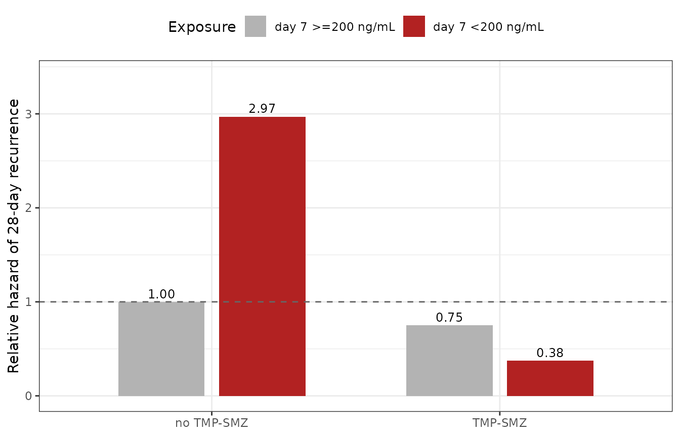
Relative hazard of 28-day recurrent parasitaemia across the four strata of Tchaparian 2016 Figure 4, at the reference covariate pattern. The reference cell is no prophylaxis with an adequate day 7 concentration.
# The direction of the interaction is the paper's headline and is a property of
# the printed coefficients, not of a draw, so it is asserted directly.
stopifnot(
  strata$hr[strata$tmpsmx == 0 & strata$low] > strata$hr[strata$tmpsmx == 0 & !strata$low],
  strata$hr[strata$tmpsmx == 1 & strata$low] < strata$hr[strata$tmpsmx == 1 & !strata$low]
)
Day 3 is the stronger predictor
The paper’s comparative analysis reports that in children without
prophylaxis, a one-unit rise in natural-log concentration reduces the
28-day hazard by 49% on day 3 but only 20% on day 7. The two outputs
hr_c3 and hr_c7 carry those two fits as
exposure-only relative hazards, in which the unprinted adjustment terms
cancel.
ratio_of <- function(col, ref_val) {
  row <- ref_row
  row[[col]] <- ref_val * exp(1)
  out <- rxode2::rxSolve(pd, row, rxode2::et(0), returnType = "data.frame")
  if (col == "CONC_LUMEFANTRINE_72H") out$hr_c3[1] else out$hr_c7[1]
}

slope_tab <- tibble::tibble(
  Landmark = c("Day 3 (72 h)", "Day 7 (168 h)"),
  `Model HR per ln unit` = round(c(
    ratio_of("CONC_LUMEFANTRINE_72H", 2777),
    ratio_of("CONC_LUMEFANTRINE_168H", 216)
  ), 4),
  Published = c(0.51, 0.80)
)
knitr::kable(slope_tab, caption = "Hazard ratio per one-unit increase in natural-log lumefantrine concentration, children not receiving prophylaxis (Tchaparian 2016 Results and Discussion).")| Landmark | Model HR per ln unit | Published |
|---|---|---|
| Day 3 (72 h) | 0.51 | 0.51 |
| Day 7 (168 h) | 0.80 | 0.80 |
Linking the two models
The recurrence model’s exposure column is meant to be generated by the PK model, which is what makes the pair usable together. Feeding the simulated cohort’s own day 7 concentrations through the hazard model gives the exposure distribution the threshold acts on.
linked <- per_id |>
  dplyr::transmute(
    id,
    CONC_LUMEFANTRINE_168H = c168,
    CONC_LUMEFANTRINE_72H = c72,
    CONMED_TMPSMX = 0, AGE = 0.75, RESIDENCE_RURAL = 0,
    HGB = 10, PARA = 17603, WAZ = 0
  )

linked_hr <- rxode2::rxSolve(pd, linked, rxode2::et(0), returnType = "data.frame")
frac_low <- mean(linked$CONC_LUMEFANTRINE_168H < 200)

link_tab <- tibble::tibble(
  Quantity = c(
    "Children below the 200 ng/mL day 7 threshold, %",
    "Median relative hazard, no prophylaxis",
    "Median relative hazard if all were on prophylaxis"
  ),
  Value = c(
    round(100 * frac_low, 1),
    round(median(linked_hr$hr), 3),
    round(median(rxode2::rxSolve(pd, dplyr::mutate(linked, CONMED_TMPSMX = 1),
      rxode2::et(0), returnType = "data.frame")$hr), 3)
  )
)
knitr::kable(link_tab, caption = "The PK model feeding the recurrence model, reference covariate pattern otherwise.")| Quantity | Value |
|---|---|
| Children below the 200 ng/mL day 7 threshold, % | 47.50 |
| Median relative hazard, no prophylaxis | 1.00 |
| Median relative hazard if all were on prophylaxis | 0.75 |
# The paper's measured day 7 median of 216 ng/mL sits just above the 200 ng/mL
# threshold, so roughly half the cohort should fall below it. A wide bound: the
# quantity is a proportion of a random cohort near a threshold, and the bound
# still fails if the exposure distribution is off by the factor that a
# mis-transcribed dose or clearance would produce.
stopifnot(frac_low > 0.2, frac_low < 0.7)
Assumptions and deviations
Day 3 concentrations run about 15% above the measured median,
reproducibly. Across 1, 2, 4, 8 and 16 solver threads the
simulated day 3 median was +14.1% to +17.3% against the measured 2777
ng/mL, while every other comparison sat within 7%. This is recorded as a
deviation rather than absorbed into a wider bound. The likely mechanism
is named by the paper itself: “the lack of sufficient sampling times
during the absorption phase, making it difficult to detect an absorption
delay and related kinetics”, which is also why ka was fixed
to 0.45 1/h from a different study rather than estimated. Day 3 is 12 h
after the last dose and closest to the peak, so it is precisely where an
unmodelled absorption lag would bias predictions upward. Note also that
the published 2777 ng/mL is a measured median carrying assay
variability and real home-dosing times, whereas the simulated value is a
noise-free individual prediction at exactly 72 h.
The model’s formal terminal half-life is far longer than
lumefantrine’s accepted value. V2/F of 441 L with
Q/F of 0.23 L/h implies a beta half-life near 60 days,
against the roughly 4.5 days the paper’s own Introduction quotes for
lumefantrine. This is a faithful transcription, not an error:
V2/F carries an RSE of 74% and the deep compartment holds
very little mass, so the observable decline is much faster and
does match the paper – the typical child crosses the LOD at 9.6 days
against the paper’s “approximately 10 days”. The practical consequence
is narrower than it first appears: PKNCA’s span ratio over a 1512 h
window is 0.65 to 0.78, so lambda.z is fitted to a phase
the window does not fully cover, yet the extrapolated
aucinf.obs still lands within about 0.1% of
F * Dose / CL. Users sampling over a materially shorter
window should not assume that continues to hold.
The base of the parasite-density logarithm is
inferred. Methods describe the Table 3 covariate only as
“parasite density (log transformed)” without naming a base. The natural
log is used here because the same paper names natural log explicitly for
the day 3 and day 7 concentration analyses one subsection later. A log10
reading would rescale e_para_haz by ln(10),
making the effect 2.30 times steeper per log10 unit; the covariate is
not significant either way (HR 1.04, 95% CI 0.95-1.14, P = .35), so the
choice does not affect any published conclusion, but a user fitting this
term to new data should confirm the base.
Centring values for the two continuous Cox covariates are the
cohort summaries, not published reference values. The paper
prints per-unit hazard ratios for haemoglobin and parasite density but
no centring value. Haemoglobin is centred on the Table 1 median (10.0
g/dL) and parasite density on the Table 1 geometric mean (17,603
parasites/uL), so that hr is 1 at a typical child. This is
presentational only: every hazard ratio between two covariate
values is unchanged by the choice.
The prophylaxis main effect and the exposure effect are not printed on one consistent parameterisation. Table 3 gives the low-exposure effect within each prophylaxis stratum (2.97 and 0.50) because the interaction is significant, but lists the prophylaxis effect (0.75) in the main-effect block, where the day-7-concentration row reads 1.21 rather than the 2.97 the interaction model implies. The two blocks therefore come from different fits, and the prophylaxis coefficient in the interaction model is not identifiable from the table. The model uses 0.75 as the prophylaxis effect within the adequate-exposure stratum and flags it here. The direction is corroborated twice independently: the prophylaxis stratum had a higher adequate-response rate (65.9% versus 59.1%) and the Discussion attributes the attenuated exposure-response to “the independent protective effects of TMP-SMZ against malaria”. The marginal 1.21 row is not encoded, since it contradicts the retained interaction model.
Coincidence warning on the value 1.21. Table 3
prints 1.21 twice, once for rural residence (95% CI 0.43-3.43) and once
for the day-7-concentration main effect (95% CI 0.71-2.07).
e_residence_rural_haz is the residence row. The two must
not be conflated.
No baseline hazard, by construction. A Cox
regression is semiparametric, so h0(t) was never produced
by the fit; the recurrence model returns relative hazards only and
offers no survivor function. Figure 4 and Supplemental Figure S3 carry
the paper’s empirical Kaplan-Meier description of the absolute time
course.
Interoccasion variability is encoded for five
occasions. Monolix reports one interoccasion magnitude per
parameter shared across occasions, so occasion 1 carries the estimated
variance and occasions 2 to 5 repeat it through fixed(),
following Stoschus_2025_phenobarbital and
Ding_2026_vancomycin. Five spans the observed maximum
episodes per child (Table 1). Simulations here use OCC = 1.
This encoding raises a non-mu-referenced eta warning from rxode2 at
parse time, which is inherent to indicator-multiplexed interoccasion
variability and is shared by both registered precedents; it affects
estimation, not simulation.
Left censoring is not reproduced. The fit retained 188 below-LOD samples (23.3%) as left-censored, which is what informs the 14-day tail. The simulations here are uncensored, so simulated concentrations below 52 ng/mL appear as real values where the study could only record a censoring event.
Race and ethnicity are not reported beyond the cohort being Ugandan children resident in Tororo district, and are not covariates in either model.
Cohort construction. Weight and age were calibrated to the Table 1 marginals rather than drawn from WHO growth curves, because the published exposure summaries are conditioned on this cohort’s own distributions and the cohort runs below the WHO median for age (reported median weight-for-age z score -0.74).