Gentamicin in neonates undergoing therapeutic hypothermia (van der Veer 2024)
Source:vignettes/articles/vanderVeer_2024_gentamicin.Rmd
vanderVeer_2024_gentamicin.RmdModel and source
- Citation: van der Veer MAA, de Haan TR, Franken LGW, Groenendaal F, Dijk PH, de Boode WP, Simons S, Dijkman KP, van Straaten HLM, Rijken M, Cools F, Nuytemans DHGM, van Kaam AH, Bijleveld YA, Mathot RAA. Predictive Performance of a Gentamicin Pharmacokinetic Model in Term Neonates with Perinatal Asphyxia Undergoing Controlled Therapeutic Hypothermia. Ther Drug Monit. 2024;46(3):376.
- Article: https://doi.org/10.1097/FTD.0000000000001166
- Original model: Bijleveld YA et al. Br J Clin Pharmacol.
2016;81:1067-1077 (https://doi.org/10.1111/bcp.12883), packaged as
Bijleveld_2016_gentamicin.
mod <- readModelDb("vanderVeer_2024_gentamicin")
mod_meta <- rxode2::rxode(mod)
#> ℹ parameter labels from comments will be replaced by 'label()'
mod_meta$description
#> [1] "Two-compartment population PK model of intravenous gentamicin in (near-)term neonates with perinatal asphyxia undergoing controlled therapeutic hypothermia, refitted by van der Veer 2024 to the merged model-building plus external-validation PharmaCool data set (original structure Bijleveld 2016): fixed allometric body-weight scaling (0.75 on CL and Q, 1 on Vc and Vp), a gestational-age power effect on CL, a study-day-5 (> 96 h postnatal age) multiplicative increase in CL, and inter-individual variability on the log-scale residual error."
mod_meta$units
#> $time
#> [1] "h"
#>
#> $dosing
#> [1] "mg"
#>
#> $concentration
#> [1] "mg/L"
van der Veer 2024 externally validated the Bijleveld 2016 gentamicin
model on 39 new neonates from the PharmaCool Study. The model predicted
the new data well, so the authors merged the model-building and external
data sets and re-estimated the same structural, covariate and
variability model on all 86 neonates (Table 2, “Refit: Merged Data
Set”). This package entry is that refit; the original fit remains
available as Bijleveld_2016_gentamicin.
Population
The merged data set holds 86 (near-)term neonates (GA > 36 weeks) with perinatal asphyxia treated with controlled therapeutic hypothermia in 10 Dutch and 2 Belgian NICUs, with 935 gentamicin concentrations (612 model-building plus 323 external; Table 1). Gestational age was median 40 weeks (range 36-42) in both sets; birth weight median 3.40 kg (2.09-5.07) in the model-building set and 3.17 kg (2.26-4.62) in the external set; 49 of 86 neonates were male. Gentamicin was given as 30-minute infusions of 4 mg/kg every 24 h (daily dose 3.0-5.9 mg/kg), with concentration-guided adjustment. Samples were drawn during hypothermia (days 2-3), rewarming (day 4) and normothermia (day 5).
str(mod_meta$population)
#> List of 12
#>  $ species       : chr "human"
#>  $ n_subjects    : int 86
#>  $ n_studies     : int 1
#>  $ n_observations: int 935
#>  $ ga_range      : chr "36-42 weeks (median 40 in both data sets)"
#>  $ weight_range  : chr "2.09-5.07 kg birth weight (medians 3.40 and 3.17 kg in the two data sets)"
#>  $ pna_range     : chr "1.5-5.2 days at end of study (medians 4.7 and 3.1 days in the two data sets)"
#>  $ sex_female_pct: num 43
#>  $ disease_state : chr "(Near-)term neonates (GA > 36 weeks) with perinatal asphyxia meeting the criteria for controlled therapeutic hy"| __truncated__
#>  $ dose_range    : chr "Gentamicin 30-min IV infusions of 4 mg/kg every 24 h, with concentration-guided adjustment per local protocol; "| __truncated__
#>  $ regions       : chr "10 Dutch and 2 Belgian neonatal intensive care units (PharmaCool Study, NTR2529)."
#>  $ notes         : chr "Merged data set = the 47-neonate / 612-sample model-building set of Bijleveld 2016 plus a 39-neonate / 323-samp"| __truncated__
Source trace
| Equation / parameter | Value | Source location |
|---|---|---|
lcl (CL per 70 kg) |
log(1.88) L/h | Table 2, Refit: Merged Data Set |
lvc (Vc per 70 kg) |
log(33.2) L | Table 2, Refit: Merged Data Set |
lq (Q per 70 kg) |
log(1.81) L/h | Table 2, Refit: Merged Data Set |
lvp (Vp per 70 kg) |
log(32.2) L | Table 2, Refit: Merged Data Set |
e_wt_cl_q |
0.75 (fixed) | Table 2 footnote, final-model equations |
e_wt_vc_vp |
1 (fixed) | Table 2 footnote, final-model equations |
e_ga_cl (theta_CLGA) |
2.76 | Table 2, Refit: Merged Data Set |
e_sd5_cl (theta_SD5) |
1.36 | Table 2, Refit: Merged Data Set; footnote “study day 5 (>96 h postnatal age)” |
| IIV CL | 24.5% -> omega^2 = 0.0582925 | Table 2, Refit: Merged Data Set |
| IIV Vc | 30.1% -> omega^2 = 0.0867289 | Table 2, Refit: Merged Data Set |
| IIV Vp | 56.4% -> omega^2 = 0.276188 | Table 2, Refit: Merged Data Set |
| Cor(CL, Vc) | 0.81 -> covariance 0.0575935 | Not reported in the refit; carried from Bijleveld 2016 Results |
expSd |
0.16 | Table 2, Refit: Merged Data Set (“Additive error”, on log-transformed data) |
etaexpSd (IIV on residual error) |
52.3% -> omega^2 = 0.241792 | Table 2, Refit: Merged Data Set |
| CL = CL x (BW/70)^0.75 x theta_SD5 x (GA/GAmedian)^theta_CLGA | n/a | Table 2 footnote |
| Vc, Vp = V x (BW/70); Q = Q x (BW/70)^0.75 | n/a | Table 2 footnote |
| GAmedian = 40 weeks | n/a | Table 1 (median GA of both data sets) |
| Two-compartment IV model | n/a | Methods, “Original Model” |
Refit versus original fit
The authors judged a refitted parameter accurate if it differed by less than 20% from the original fit. The table compares the typical values of the two packaged models.
theta_of <- function(m) {
  th <- rxode2::rxode(m)$theta
  data.frame(parameter = names(th), value = unname(th))
}
param_cmp <- dplyr::inner_join(
  theta_of(readModelDb("Bijleveld_2016_gentamicin")),
  theta_of(mod),
  by = "parameter",
  suffix = c("_original", "_refit")
) |>
  dplyr::filter(!grepl("^e_wt", parameter)) |>
  dplyr::mutate(
    original = ifelse(grepl("^l", parameter), exp(value_original), value_original),
    refit = ifelse(grepl("^l", parameter), exp(value_refit), value_refit),
    pct_diff = 100 * (refit - original) / original,
    parameter = ifelse(grepl("^l", parameter), sub("^l", "", parameter), parameter)
  )
#> ℹ parameter labels from comments will be replaced by 'label()'
#> ℹ parameter labels from comments will be replaced by 'label()'

param_cmp |>
  dplyr::select(parameter, original, refit, pct_diff) |>
  dplyr::rename(
    "Parameter" = parameter,
    "Bijleveld 2016" = original,
    "van der Veer 2024 refit" = refit,
    "Difference (%)" = pct_diff
  ) |>
knitr::kable(digits = 3)| Parameter | Bijleveld 2016 | van der Veer 2024 refit | Difference (%) |
|---|---|---|---|
| cl | 1.89 | 1.88 | -0.529 |
| vc | 32.50 | 33.20 | 2.154 |
| q | 2.01 | 1.81 | -9.950 |
| vp | 30.30 | 32.20 | 6.271 |
| e_ga_cl | 3.00 | 2.76 | -8.000 |
| e_sd5_cl | 1.29 | 1.36 | 5.426 |
| expSd | 0.15 | 0.16 | 6.667 |
Virtual cohort
Observed data are not public. The virtual cohort draws birth weight from a log-normal distribution centred on the merged-cohort median (about 3.3 kg, truncated to the observed 2.09-5.07 kg range) and gestational age from 36-42 weeks weighted towards 40 weeks. Each neonate receives one 4 mg/kg dose as a 30-minute infusion at 6 h postnatal age, which is the standard regimen in both data sets. Postnatal age is supplied on every row (in months) so the study-day-5 step would fire at 96 h; with sampling to 72 h after the dose it stays inside the hypothermia and rewarming window.
set.seed(20241166)
rxode2::rxSetSeed(20241166)

n_sub <- 200L
hours_per_month <- 24 * 30.4375
first_dose_pna_h <- 6

cohort <- data.frame(
  id = seq_len(n_sub),
  WT = pmin(pmax(exp(rnorm(n_sub, log(3.3), 0.17)), 2.09), 5.07),
  GA = sample(36:42, n_sub, replace = TRUE, prob = c(1, 2, 4, 5, 5, 3, 1))
)

obs_times <- sort(unique(c(0, seq(0.25, 2, by = 0.25), seq(3, 72, by = 1))))

single_events <- dplyr::bind_rows(
  cohort |>
    dplyr::mutate(time = 0, evid = 1L, amt = 4 * WT, rate = 4 * WT / 0.5),
  tidyr::expand_grid(cohort, time = obs_times) |>
    dplyr::mutate(evid = 0L, amt = 0, rate = 0)
) |>
  dplyr::mutate(
    cmt = "central",
    PNA = (first_dose_pna_h + time) / hours_per_month,
    treatment = "4 mg/kg single dose"
  ) |>
  dplyr::arrange(id, time, dplyr::desc(evid))
Simulation
sim_single <- rxode2::rxSolve(
  mod,
  events = single_events,
  keep = c("WT", "GA", "treatment")
) |>
  as.data.frame()
#> ℹ parameter labels from comments will be replaced by 'label()'
Concentration-time profile after a dose (cf. Figure 4)
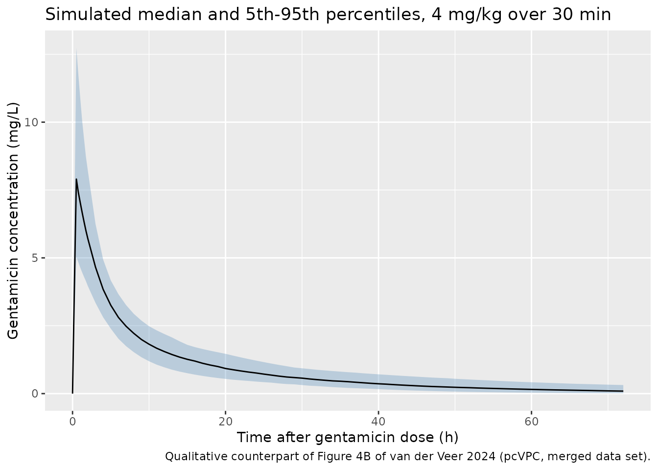
Figure 4B of van der Veer 2024 is a prediction-corrected VPC of the merged data set against time after dose. A pcVPC normalises each observation to the population prediction of its bin, so the simulated percentiles below (no prediction correction, a single 4 mg/kg dose) are only a qualitative counterpart: the median falls from about 5-6 mg/L just after the infusion to below 1 mg/L by 24-36 h, as in the figure.
sim_single |>
  dplyr::group_by(time) |>
  dplyr::summarise(
    p05 = quantile(Cc, 0.05),
    p50 = median(Cc),
    p95 = quantile(Cc, 0.95),
    .groups = "drop"
  ) |>
  ggplot(aes(time, p50)) +
  geom_ribbon(aes(ymin = p05, ymax = p95), alpha = 0.3, fill = "steelblue") +
  geom_line() +
  labs(
    x = "Time after gentamicin dose (h)",
    y = "Gentamicin concentration (mg/L)",
    title = "Simulated median and 5th-95th percentiles, 4 mg/kg over 30 min",
    caption = "Qualitative counterpart of Figure 4B of van der Veer 2024 (pcVPC, merged data set)."
  )
Recommended dosing regimens
The paper concludes that the refit supports the Bijleveld 2016 regimens of 5 mg/kg every 36 h for GA 36-41 weeks and every 24 h for GA 42 weeks, aimed at a peak of 8-12 mg/L and a trough below 1 mg/L. The typical-value profiles for a 3 kg neonate are shown for both the refit and the original fit, over 7 days starting at 6 h postnatal age so the study-day-5 increase in CL (at 96 h postnatal age) is visible.
regimens <- data.frame(
  regimen = c("GA 36 wk, 5 mg/kg q36h", "GA 40 wk, 5 mg/kg q36h", "GA 42 wk, 5 mg/kg q24h"),
  GA = c(36, 40, 42),
  interval = c(36, 36, 24)
)
duration_h <- 7 * 24
reg_times <- sort(unique(c(seq(0, duration_h, by = 0.25))))

make_regimen <- function(i) {
  r <- regimens[i, ]
  dose_times <- seq(0, duration_h - 1, by = r$interval)
  dplyr::bind_rows(
    data.frame(time = dose_times, evid = 1L, amt = 5 * 3, rate = 5 * 3 / 0.5),
    data.frame(time = reg_times, evid = 0L, amt = 0, rate = 0)
  ) |>
    dplyr::mutate(
      id = i,
      cmt = "central",
      WT = 3,
      GA = r$GA,
      PNA = (first_dose_pna_h + time) / hours_per_month,
      regimen = r$regimen
    )
}
reg_events <- dplyr::bind_rows(lapply(seq_len(nrow(regimens)), make_regimen)) |>
  dplyr::arrange(id, time, dplyr::desc(evid))

sim_reg <- dplyr::bind_rows(
  rxode2::rxSolve(rxode2::zeroRe(mod), events = reg_events, keep = "regimen") |>
    as.data.frame() |>
    dplyr::mutate(model = "van der Veer 2024 refit"),
  rxode2::rxSolve(
    rxode2::zeroRe(readModelDb("Bijleveld_2016_gentamicin")),
    events = reg_events, keep = "regimen"
  ) |>
    as.data.frame() |>
    dplyr::mutate(model = "Bijleveld 2016 original")
)
#> ℹ parameter labels from comments will be replaced by 'label()'
#> Warning: No sigma parameters in the model
#> ℹ omega/sigma items treated as zero: 'etalcl', 'etalvc', 'etalvp', 'etaexpSd'
#> Warning: multi-subject simulation without without 'omega'
#> ℹ parameter labels from comments will be replaced by 'label()'
#> ℹ omega/sigma items treated as zero: 'etalcl', 'etalvc', 'etalvp'
#> Warning: multi-subject simulation without without 'omega'

ggplot(sim_reg, aes(time, Cc, colour = model)) +
  annotate("rect", xmin = -Inf, xmax = Inf, ymin = 8, ymax = 12, alpha = 0.15, fill = "steelblue") +
  geom_hline(yintercept = 1, linetype = "dashed") +
  geom_vline(xintercept = 96 - first_dose_pna_h, linetype = "dotted") +
  geom_line() +
  facet_wrap(~regimen, ncol = 1) +
  scale_x_continuous(breaks = seq(0, 168, 24)) +
  labs(
    x = "Time after first dose (h)",
    y = "Gentamicin concentration (mg/L)",
    colour = NULL,
    caption = paste(
      "Typical 3 kg neonate. Shaded band: 8-12 mg/L peak target; dashed line:",
      "1 mg/L trough target; dotted line: 96 h postnatal age (study day 5)."
    )
  ) +
  theme(legend.position = "bottom")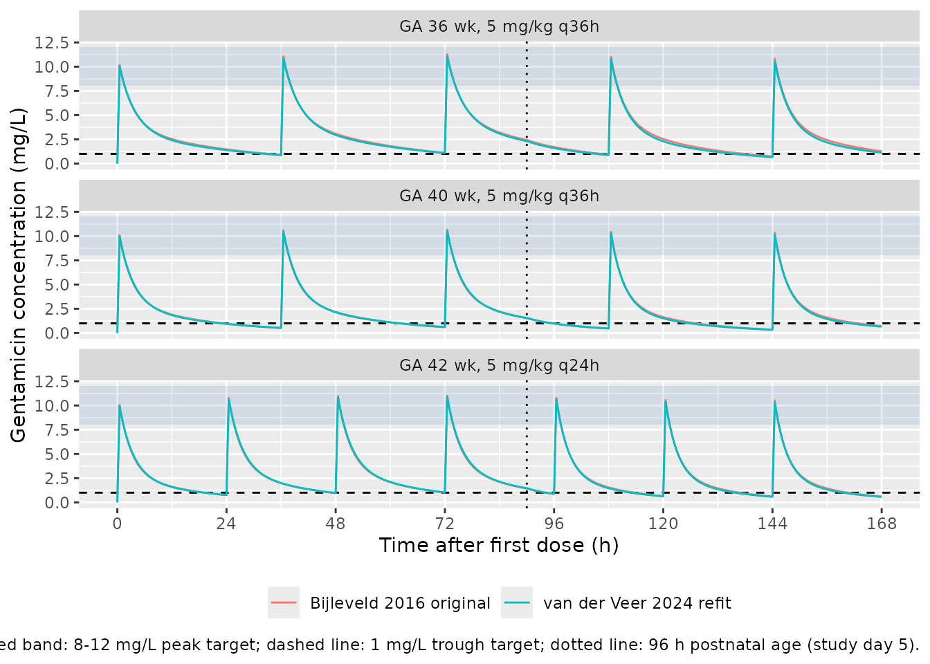
peak_trough <- dplyr::bind_rows(lapply(seq_len(nrow(regimens)), function(i) {
  r <- regimens[i, ]
  dose_times <- seq(0, duration_h - r$interval, by = r$interval)
  sim_reg |>
    dplyr::filter(regimen == r$regimen) |>
    dplyr::group_by(model) |>
    dplyr::summarise(
      regimen = r$regimen,
      peak_first = Cc[time == 1],
      trough_first = Cc[time == r$interval],
      .groups = "drop"
    )
}))

peak_trough |>
  dplyr::select(regimen, model, peak_first, trough_first) |>
  dplyr::rename(
    "Regimen" = regimen,
    "Model" = model,
    "Peak 30 min after first infusion (mg/L)" = peak_first,
    "Trough before second dose (mg/L)" = trough_first
  ) |>
knitr::kable(digits = 2)| Regimen | Model | Peak 30 min after first infusion (mg/L) | Trough before second dose (mg/L) |
|---|---|---|---|
| GA 36 wk, 5 mg/kg q36h | Bijleveld 2016 original | 9.13 | 0.90 |
| GA 36 wk, 5 mg/kg q36h | van der Veer 2024 refit | 9.03 | 0.87 |
| GA 40 wk, 5 mg/kg q36h | Bijleveld 2016 original | 8.89 | 0.51 |
| GA 40 wk, 5 mg/kg q36h | van der Veer 2024 refit | 8.82 | 0.52 |
| GA 42 wk, 5 mg/kg q24h | Bijleveld 2016 original | 8.76 | 0.76 |
| GA 42 wk, 5 mg/kg q24h | van der Veer 2024 refit | 8.70 | 0.76 |
refit_targets <- dplyr::filter(peak_trough, model == "van der Veer 2024 refit")
# Typical-value check of the paper's conclusion: every recommended regimen
# reaches the 8-12 mg/L peak window and stays below the 1 mg/L trough.
stopifnot(
  all(refit_targets$peak_first > 8 & refit_targets$peak_first < 12),
  all(refit_targets$trough_first < 1)
)
PKNCA validation
Single-dose NCA of the stochastic cohort, grouped by treatment. The paper reports no NCA parameters, so there is no published comparison; instead, a typical-value solve checks that AUC0-inf equals dose / CL.
conc_df <- sim_single |>
  dplyr::filter(!is.na(Cc)) |>
  dplyr::select(id, time, Cc, treatment)
dose_df <- single_events |>
  dplyr::filter(evid == 1L) |>
  dplyr::select(id, time, amt, treatment)

conc_obj <- PKNCA::PKNCAconc(conc_df, Cc ~ time | treatment + id, concu = "mg/L", timeu = "h")
dose_obj <- PKNCA::PKNCAdose(dose_df, amt ~ time | treatment + id, doseu = "mg", route = "intravascular", duration = 0.5)
intervals <- data.frame(
  start = 0, end = Inf,
  cmax = TRUE, tmax = TRUE, aucinf.obs = TRUE, half.life = TRUE
)
nca_res <- PKNCA::pk.nca(PKNCA::PKNCAdata(conc_obj, dose_obj, intervals = intervals))
summary(nca_res)
#>  Interval Start Interval End           treatment   N Cmax (mg/L)
#>               0          Inf 4 mg/kg single dose 200 7.97 [29.2]
#>              Tmax (h) Half-life (h) AUCinf,obs (h*mg/L)
#>  0.500 [0.500, 0.500]   18.2 [8.96]         72.6 [26.8]
#>
#> Caption: Cmax, AUCinf,obs: geometric mean and geometric coefficient of variation; Tmax: median and range; Half-life: arithmetic mean and standard deviation; N: number of subjects
# Typical 3 kg, 40-week neonate, 12 mg (4 mg/kg) over 30 min, sampled to
# 400 h; postnatal age held below 96 h so CL is constant.
typ_events <- dplyr::bind_rows(
  data.frame(time = 0, evid = 1L, amt = 12, rate = 24),
  data.frame(time = c(0, seq(0.25, 2, by = 0.25), seq(3, 400, by = 1)), evid = 0L, amt = 0, rate = 0)
) |>
  dplyr::mutate(id = 1L, cmt = "central", WT = 3, GA = 40, PNA = 1 / hours_per_month)
typ <- rxode2::rxSolve(rxode2::zeroRe(mod), events = typ_events) |>
  as.data.frame() |>
  dplyr::mutate(id = 1L)
#> ℹ parameter labels from comments will be replaced by 'label()'
#> Warning: No sigma parameters in the model
#> ℹ omega/sigma items treated as zero: 'etalcl', 'etalvc', 'etalvp', 'etaexpSd'
nca_typ <- PKNCA::pk.nca(PKNCA::PKNCAdata(
  PKNCA::PKNCAconc(typ, Cc ~ time | id),
  PKNCA::PKNCAdose(data.frame(id = 1L, time = 0, amt = 12), amt ~ time | id, route = "intravascular", duration = 0.5),
  intervals = data.frame(start = 0, end = Inf, aucinf.obs = TRUE)
))
auc_nca <- as.data.frame(nca_typ$result) |>
  dplyr::filter(PPTESTCD == "aucinf.obs") |>
  dplyr::pull(PPORRES)
cl_typ <- 1.88 * (3 / 70)^0.75
c(AUCinf_NCA = auc_nca, dose_over_CL = 12 / cl_typ)
#>   AUCinf_NCA dose_over_CL
#>     67.79417     67.76508
# Same parameters on both sides: only trapezoidal error separates them.
stopifnot(abs(auc_nca / (12 / cl_typ) - 1) < 0.02)
Assumptions and deviations
- CL-Vc correlation carried from the original fit. The refit (Table 2) reports the IIV of CL and Vc but not their correlation. The original Bijleveld 2016 model estimated r = 0.81, and the refit re-estimated the same model, so r = 0.81 is carried forward to form the covariance.
-
IIV converted with omega^2 = log(1 + CV^2). Table 2
gives IIV as %CV without stating the conversion; the log-normal form is
used, as in
Bijleveld_2016_gentamicin. -
Residual error. “Additive error” 0.16 is additive
on log-transformed concentrations (the original model), encoded as
lnorm(expSd). The 52.3% IIV on the residual error is encoded as a subject-level multiplierexpSd * exp(etaexpSd). (The packaged original-fit model omits this term.) -
Study-day-5 step. theta_SD5 applies when postnatal
age exceeds 96 h (Table 2 footnote); the model derives the indicator
from the canonical
PNAcolumn (months). - GA reference. “GAmedian” is taken as 40 weeks, the median of both data sets in Table 1.
- Body weight. The allometric covariate is birth weight held constant over the simulation window, as in the source.
- Virtual cohort. Weight and gestational age distributions are approximations matched to the Table 1 medians and ranges; each subject gets one 4 mg/kg dose at 6 h postnatal age.
- Errata. No erratum for this article was found when it was added (2026-10-29).