Enoxaparin anti-factor Xa (SanchezPena 2005)
Source:vignettes/articles/SanchezPena_2005_enoxaparin.Rmd
SanchezPena_2005_enoxaparin.RmdModel and source
- Citation: Sanchez-Pena P, Hulot JS, Urien S, Ankri A, Collet JP, Choussat R, Lechat P, Montalescot G. Anti-factor Xa kinetics after intravenous enoxaparin in patients undergoing percutaneous coronary intervention: a population model analysis. British Journal of Clinical Pharmacology 2005; 60(4):364-373. doi:[10.1111/j.1365-2125.2005.02452.x](https://doi.org/10.1111/j.1365-2125.2005.02452.x).
- Full text (Open Access via PMC): https://pmc.ncbi.nlm.nih.gov/articles/PMC1884774/.
This is a one-compartment population PK model of anti-factor Xa activity after a single IV bolus of enoxaparin in adult patients undergoing elective percutaneous coronary intervention (PCI). The IV bolus is described by a short zero-order input phase (duration T0) into the central compartment with linear elimination. Body weight is the only retained covariate, applied as separately estimated allometric exponents on clearance (0.9) and volume (0.7) with a reference weight of 75 kg. A fixed endogenous basal anti-Xa activity (0.0725 IU/mL) is added to the dose-driven prediction to account for the chromogenic assay’s non-zero pre-dose reading.
mod_fn  <- readModelDb("SanchezPena_2005_enoxaparin")
mod     <- rxode2::rxode2(mod_fn())
mod_typ <- rxode2::rxode2(rxode2::zeroRe(mod_fn()))
Population
The model was developed from 546 consecutive adult patients (mean age 63 years, range 21-93; 79% male) referred for elective PCI of coronary or vein-graft stenosis greater than 70% at a single centre (Pitie-Salpetriere University Hospital, Paris). Mean body weight was 76 kg (range 35-153). Renal function was distributed as CrCl < 30 mL/min in 4% of patients, 31-59 mL/min in 33%, and >= 60 mL/min in 62%; 15% of patients were aged > 75 years. Concomitant GPIIb/IIIa inhibitors were used in 175 patients (146 eptifibatide, 29 abciximab); all patients received a 500 mg IV loading dose of aspirin followed by 75 mg/day orally.
Each patient received a single 0.5 mg/kg IV bolus of enoxaparin (mean dose 38 +/- 7 mg = 3830 +/- 730 IU) immediately before PCI. Five samples were drawn per patient: pre-bolus, 10 min post-bolus (start of PCI), end of PCI (mean 45 min), 3 h post-PCI, and the morning after PCI. Out of 556 enrolled, 10 (1.8%) were excluded for probable misadministration, leaving 546 patients and 1978 anti-Xa concentrations. Demographics in Sanchez-Pena 2005 Table 1.
The same information is available programmatically via
readModelDb("SanchezPena_2005_enoxaparin")$population.
Source trace
Per-parameter origins are recorded as in-file comments in
inst/modeldb/specificDrugs/SanchezPena_2005_enoxaparin.R;
the table below collects them in one place for review.
| Item | Value (typical) | Source |
|---|---|---|
| One-compartment disposition with zero-order IV input | structural | Results, Population pharmacokinetics: “best described by a one-compartment model with zero-order input” |
lcl -> TV.CL = 1.20 L/h |
1.20 | Table 2 (mean +/- SE 1.20 +/- 0.03; bootstrap median 1.17) |
lvc -> TV.V = 2.9 L |
2.9 | Table 2 (2.9 +/- 0.1; bootstrap median 2.9) |
tdur -> T0 = 0.25 h |
0.25 | Table 2 (0.25 +/- 0.01; bootstrap median 0.24) |
e_wt_cl -> BW exponent on CL |
0.9 | Table 2 (0.9 +/- 0.1) |
e_wt_vc -> BW exponent on V |
0.7 | Table 2 (0.7 +/- 0.1) |
| Reference body weight (BW for covariate equation) | 75 kg | Results, page above Table 2: CL = TV_CL * (BW/75)^0.9,
V = TV_V * (BW/75)^0.7
|
bl_antiXa -> Basal anti-Xa (FIXED) |
0.0725 IU/mL | Table 2 (“Basal anti-Xa (IU/mL): 0.0725 (fixed)”) |
etalcl -> ISV on CL |
33% CV | Table 2 (33 +/- 3 %CV); var on log scale = log(0.33^2 + 1) = 0.10336 |
etalvc -> ISV on V |
30% CV | Table 2 (30 +/- 7 %CV); var on log scale = log(0.30^2 + 1) = 0.08618 |
etatdur -> ISV on T0 (additive) |
0.06 h SD | Table 2 (0.06 +/- 0.02 h, additive error model); var = 0.0036 |
addSd -> Residual SD (additive) |
0.09 IU/mL | Table 2 (0.09 +/- 0.02 IU/mL, additive error model) |
Virtual cohort
The original observed data are not publicly available. The simulations below use a virtual cohort whose body-weight distribution approximates the published demographics (mean 76 kg, SD 15 kg, truncated to the 35-153 kg range). Three dose levels are simulated to match the paper’s Figure 3 panels (0.5, 0.75, and 1 mg/kg single IV bolus).
set.seed(20251104L)

n_per_dose <- 300L
dose_levels <- c("0.5 mg/kg" = 0.5,
                 "0.75 mg/kg" = 0.75,
                 "1 mg/kg" = 1.0)

# IU per mg of enoxaparin (paper: 38 mg = 3830 IU -> 100 IU/mg). The model's
# dosing unit is anti-factor-Xa IU (see units$dosing in the model file).
IU_PER_MG <- 100

obs_times <- c(0,
               seq(0.05, 0.5, by = 0.05),
               seq(0.6, 12, by = 0.2))

build_subjects <- function(n, dose_mg_per_kg, dose_label, id_offset = 0L) {
  wt <- pmin(pmax(stats::rnorm(n, mean = 76, sd = 15), 35), 153)
  tibble::tibble(
    id          = id_offset + seq_len(n),
    dose_label  = factor(dose_label, levels = names(dose_levels)),
    WT          = wt,
    dose_mg     = dose_mg_per_kg * wt,
    dose_IU     = dose_mg_per_kg * wt * IU_PER_MG
  )
}

build_events <- function(subjects, obs_times) {
  dose_rows <- subjects |>
    dplyr::transmute(
      id, time = 0, evid = 1L,
      amt        = dose_IU,
      cmt        = "central",
      rate       = -2,  # model-defined duration (dur(central) <- tdur_i)
      dose_label, WT
    )
  obs_rows <- tidyr::expand_grid(id = subjects$id, time = obs_times) |>
    dplyr::left_join(dplyr::select(subjects, id, dose_label, WT), by = "id") |>
    dplyr::mutate(evid = 0L, amt = 0, cmt = "Cc", rate = 0)
  dplyr::bind_rows(dose_rows, obs_rows) |>
    dplyr::arrange(id, time, dplyr::desc(evid))
}

subjects <- dplyr::bind_rows(
  build_subjects(n_per_dose, dose_levels[["0.5 mg/kg"]],  "0.5 mg/kg",
                 id_offset = 0L),
  build_subjects(n_per_dose, dose_levels[["0.75 mg/kg"]], "0.75 mg/kg",
                 id_offset =  n_per_dose),
  build_subjects(n_per_dose, dose_levels[["1 mg/kg"]],    "1 mg/kg",
                 id_offset = 2L * n_per_dose)
)
events <- build_events(subjects, obs_times)

stopifnot(!anyDuplicated(unique(events[, c("id", "time", "evid", "cmt")])))
dplyr::glimpse(subjects)
#> Rows: 900
#> Columns: 5
#> $ id         <int> 1, 2, 3, 4, 5, 6, 7, 8, 9, 10, 11, 12, 13, 14, 15, 16, 17, …
#> $ dose_label <fct> 0.5 mg/kg, 0.5 mg/kg, 0.5 mg/kg, 0.5 mg/kg, 0.5 mg/kg, 0.5 …
#> $ WT         <dbl> 73.28089, 79.42695, 60.72469, 64.53727, 46.31612, 111.60335…
#> $ dose_mg    <dbl> 36.64045, 39.71348, 30.36234, 32.26864, 23.15806, 55.80168,…
#> $ dose_IU    <dbl> 3664.045, 3971.348, 3036.234, 3226.864, 2315.806, 5580.168,…
Simulation
Stochastic simulation (full omega / sigma) for visual predictive plots and PKNCA against the published percentile bands in the paper:
sim <- rxode2::rxSolve(
  mod,
  events = events,
  keep   = c("dose_label", "WT")
) |>
  as.data.frame()
Typical-value simulation (omega/sigma zeroed) for direct comparison with the typical predictions in Sanchez-Pena 2005 Figure 3:
typical_subjects <- tibble::tibble(
  id          = seq_along(dose_levels),
  dose_label  = factor(names(dose_levels), levels = names(dose_levels)),
  WT          = 76,
  dose_mg     = unname(dose_levels) * 76,
  dose_IU     = unname(dose_levels) * 76 * IU_PER_MG
)
typical_events <- build_events(typical_subjects, obs_times)

sim_typical <- rxode2::rxSolve(
  mod_typ,
  events = typical_events,
  keep   = c("dose_label", "WT")
) |>
  as.data.frame()
#> ℹ omega/sigma items treated as zero: 'etalcl', 'etalvc', 'etatdur'
#> Warning: multi-subject simulation without without 'omega'
Replicate published figures
Figure 3 – Anti-Xa kinetics by dose (5th, 50th, 95th percentiles)
Sanchez-Pena 2005 Figure 3a-c shows the simulated 5th, 50th, and 95th percentiles of anti-Xa activity over time after a single IV bolus of enoxaparin at three dose levels: 0.5, 0.75, and 1 mg/kg. The chunk below replicates the same VPC structure across all three doses on a single panel grid.
vpc_df <- sim |>
  dplyr::group_by(dose_label, time) |>
  dplyr::summarise(
    Q05 = stats::quantile(Cc, 0.05, na.rm = TRUE),
    Q50 = stats::quantile(Cc, 0.50, na.rm = TRUE),
    Q95 = stats::quantile(Cc, 0.95, na.rm = TRUE),
    .groups = "drop"
  )

ggplot(vpc_df, aes(time, Q50)) +
  geom_ribbon(aes(ymin = Q05, ymax = Q95), alpha = 0.25, fill = "steelblue") +
  geom_line(colour = "steelblue4", linewidth = 0.7) +
  geom_hline(yintercept = c(0.5, 0.8, 1.5, 1.8),
             linetype = "dotted", colour = "grey50") +
  facet_wrap(~ dose_label, nrow = 1) +
  scale_x_continuous(breaks = seq(0, 12, by = 2)) +
  labs(
    x = "Time after IV bolus (h)",
    y = "Anti-Xa activity (IU/mL)",
    title = "Figure 3 -- anti-Xa kinetics by IV enoxaparin dose",
    caption = paste0(
      "Replicates Figure 3a (0.5 mg/kg), 3b (0.75 mg/kg), 3c (1 mg/kg) of ",
      "Sanchez-Pena 2005. Lines: simulated 5th / 50th / 95th percentiles; ",
      "ribbon spans 5th-95th. Dotted lines mark anticoagulation thresholds ",
      "at 0.5, 0.8, 1.5, 1.8 IU/mL."
    )
  )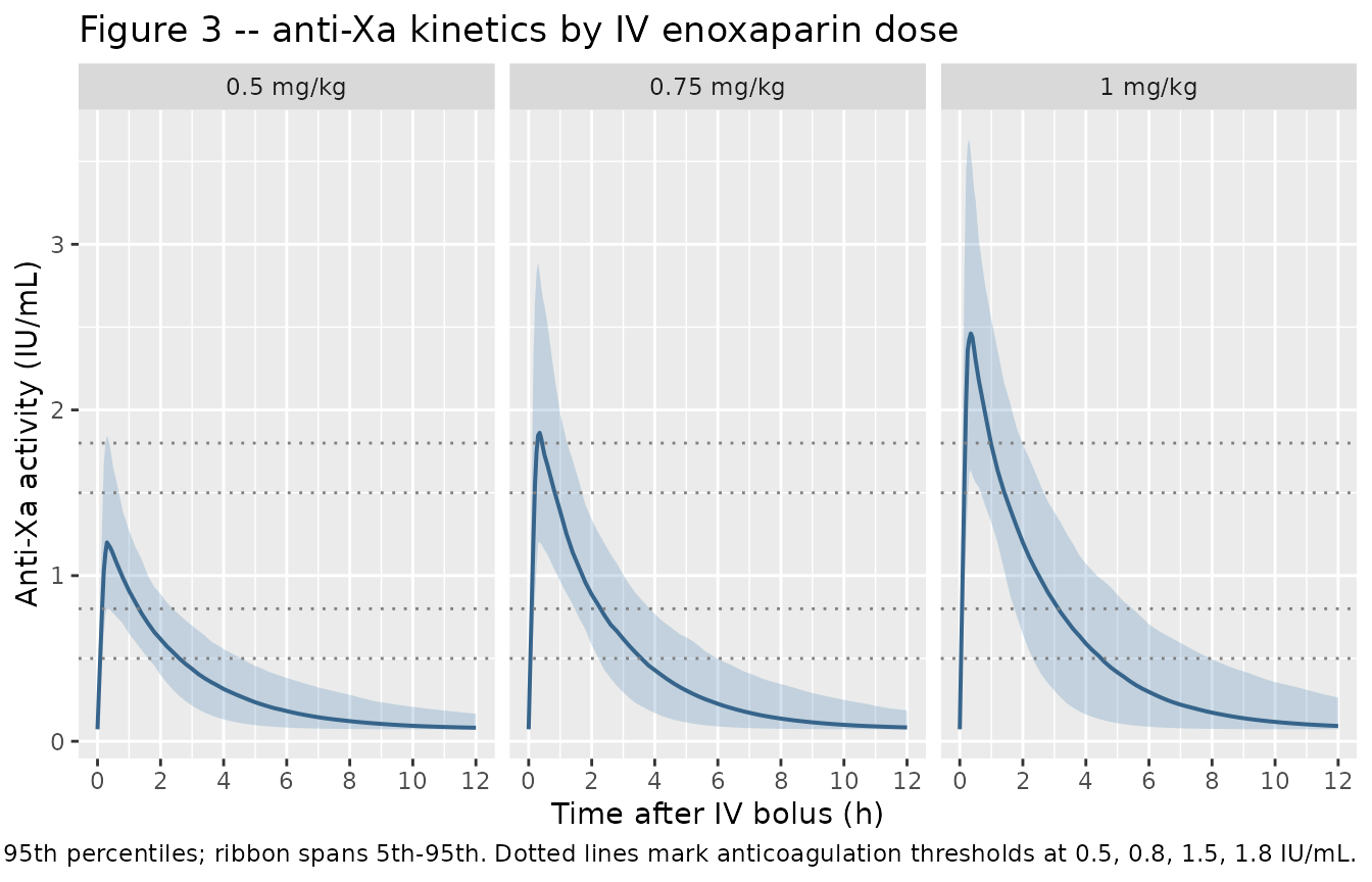
Table 3 – Patients reaching anti-Xa thresholds and mean duration
Sanchez-Pena 2005 Table 3 reports the proportion of simulated patients who reach each anticoagulation threshold (> 0.5, > 0.8, > 1.5, > 1.8 IU/mL) and the mean +/- SD duration spent above each threshold, by dose. The chunk below recomputes the same summary from the stochastic cohort. The replicated proportions and mean durations should be close to the paper’s published values (within a few percent given the finite simulation cohort).
thresholds <- c(0.5, 0.8, 1.5, 1.8)

per_subject_duration <- function(df, thr) {
  df |>
    dplyr::arrange(id, time) |>
    dplyr::group_by(id, dose_label) |>
    dplyr::summarise(
      reach    = any(Cc > thr, na.rm = TRUE),
      duration = {
        above <- Cc > thr
        if (!any(above, na.rm = TRUE)) {
          0
        } else {
          dt <- diff(time)
          # crude rectangular integration of time-above-threshold
          mid_above <- (head(above, -1) & tail(above, -1)) |
            (head(above, -1) ^ 0 & FALSE)  # only fully-above intervals
          mid_above <- head(above, -1) & tail(above, -1)
          sum(dt[mid_above], na.rm = TRUE)
        }
      },
      .groups = "drop"
    )
}

threshold_summary <- lapply(thresholds, function(thr) {
  per_subject_duration(sim, thr) |>
    dplyr::group_by(dose_label) |>
    dplyr::summarise(
      threshold      = thr,
      pct_reached    = 100 * mean(reach, na.rm = TRUE),
      dur_mean       = mean(duration[reach], na.rm = TRUE),
      dur_sd         = stats::sd(duration[reach], na.rm = TRUE),
      .groups = "drop"
    )
}) |>
  dplyr::bind_rows() |>
  dplyr::arrange(dose_label, threshold)

threshold_summary |>
  dplyr::rename(
    "Dose"              = dose_label,
    "Threshold (IU/mL)" = threshold,
    "% reaching"        = pct_reached,
    "Mean duration (h)" = dur_mean,
    "SD (h)"            = dur_sd
  ) |>
  knitr::kable(
  digits  = c(0, 1, 1, 2, 2),
  caption = paste0(
    "Replicates Sanchez-Pena 2005 Table 3. Compare against published ",
    "values: 0.5 mg/kg = 100% / 2.7 +/- 0.9 h (>0.5); 75% / 1.7 +/- 0.6 h ",
    "(>0.8); 2.5% / 0.5 +/- 0.2 h (>1.5); 0% (>1.8). ",
    "0.75 mg/kg = 100% / 3.4 +/- 1.1 h (>0.5); 100% / 2.3 +/- 0.8 h (>0.8); ",
    "48% / 1.7 +/- 0.6 h (>1.5); 28% / 1.2 +/- 0.4 h (>1.8). ",
    "1 mg/kg = 100% / 4.1 +/- 1.0 h (>0.5); 100% / 3.0 +/- 1 h (>0.8); ",
    "79% / 0.9 +/- 0.3 h (>1.5); 57% / 1.0 +/- 0.3 h (>1.8)."
  )
)| Dose | Threshold (IU/mL) | % reaching | Mean duration (h) | SD (h) |
|---|---|---|---|---|
| 0.5 mg/kg | 0.5 | 100.0 | 2.52 | 0.88 |
| 0.5 mg/kg | 0.8 | 96.7 | 1.11 | 0.58 |
| 0.5 mg/kg | 1.5 | 24.7 | 0.25 | 0.20 |
| 0.5 mg/kg | 1.8 | 7.7 | 0.14 | 0.10 |
| 0.75 mg/kg | 0.5 | 100.0 | 3.62 | 1.27 |
| 0.75 mg/kg | 0.8 | 100.0 | 2.22 | 0.82 |
| 0.75 mg/kg | 1.5 | 80.7 | 0.70 | 0.45 |
| 0.75 mg/kg | 1.8 | 56.0 | 0.48 | 0.34 |
| 1 mg/kg | 0.5 | 100.0 | 4.53 | 1.67 |
| 1 mg/kg | 0.8 | 100.0 | 3.08 | 1.10 |
| 1 mg/kg | 1.5 | 97.3 | 1.27 | 0.62 |
| 1 mg/kg | 1.8 | 88.7 | 0.87 | 0.52 |
PKNCA validation
PKNCA-based Cmax, Tmax, and AUC across the three dose levels. The
anti-Xa concentration profile is dosed in IU/mL and includes the fixed
endogenous basal component, so NCA estimates of Cmax include the
baseline; subtract bl_antiXa = 0.0725 IU/mL to compare
against the paper’s drug-only Cmax (the paper reports peaks of around
1.1 IU/mL for 0.5 mg/kg in the Bleeding complications section, and
NICE-1 / NICE-4 peaks of 1.5 +/- 0.6 IU/mL for 0.75 mg/kg and 2.1 +/-
0.7 IU/mL for 1 mg/kg in the Discussion).
sim_nca <- sim |>
  dplyr::filter(!is.na(Cc), time >= 0) |>
  dplyr::transmute(id, time, Cc, dose_label)

conc_obj <- PKNCA::PKNCAconc(sim_nca, Cc ~ time | dose_label + id)

dose_df <- subjects |>
  dplyr::transmute(id, time = 0, amt = dose_IU, dose_label)

dose_obj <- PKNCA::PKNCAdose(dose_df, amt ~ time | dose_label + id)

intervals <- data.frame(
  start      = 0,
  end        = 12,
  cmax       = TRUE,
  tmax       = TRUE,
  auclast    = TRUE,
  aucinf.obs = TRUE,
  half.life  = TRUE
)

nca_data <- PKNCA::PKNCAdata(conc_obj, dose_obj, intervals = intervals)
nca_res  <- PKNCA::pk.nca(nca_data)

nca_summary <- summary(nca_res)
knitr::kable(
  nca_summary,
  caption = paste0(
    "Simulated NCA parameters by dose group. Cmax is the observed peak ",
    "anti-Xa activity (including the 0.0725 IU/mL endogenous basal level)."
  )
)| start | end | dose_label | N | auclast | cmax | tmax | half.life | aucinf.obs |
|---|---|---|---|---|---|---|---|---|
| 0 | 12 | 0.5 mg/kg | 300 | 3.84 [23.1] | 1.24 [25.7] | 0.250 [0.100, 0.450] | 1240 [14100] | 8.99 [154] |
| 0 | 12 | 0.75 mg/kg | 300 | 5.40 [25.3] | 1.92 [28.0] | 0.300 [0.150, 0.450] | 149 [763] | 10.1 [93.0] |
| 0 | 12 | 1 mg/kg | 300 | 7.03 [28.1] | 2.52 [26.9] | 0.250 [0.100, 0.450] | 26100 [435000] | 12.5 [159] |
Comparison against published peaks
peak_sim <- sim |>
  dplyr::group_by(id, dose_label) |>
  dplyr::summarise(peak = max(Cc, na.rm = TRUE), .groups = "drop") |>
  dplyr::group_by(dose_label) |>
  dplyr::summarise(
    mean_peak    = mean(peak),
    sd_peak      = stats::sd(peak),
    median_peak  = stats::median(peak),
    .groups = "drop"
  )

peak_pub <- tibble::tibble(
  dose_label  = factor(names(dose_levels), levels = names(dose_levels)),
  published   = c("~1.1 IU/mL (mean post-hoc Cmax, Bleeding complications section)",
                  "1.5 +/- 0.6 IU/mL (NICE-1/4 anti-Xa peak, cited in Discussion)",
                  "2.1 +/- 0.7 IU/mL (NICE-1/4 anti-Xa peak, cited in Discussion)")
)

comparison <- peak_pub |>
  dplyr::left_join(peak_sim, by = "dose_label")

comparison |>
  dplyr::rename(
    "Dose"                    = dose_label,
    "Published peak (IU/mL)"  = published,
    "Simulated mean (IU/mL)"  = mean_peak,
    "Simulated SD (IU/mL)"    = sd_peak,
    "Simulated median (IU/mL)" = median_peak
  ) |>
  knitr::kable(
    digits = 2,
    caption = "Comparison of simulated mean / median peak anti-Xa activity (including basal level) against published reference peaks."
)| Dose | Published peak (IU/mL) | Simulated mean (IU/mL) | Simulated SD (IU/mL) | Simulated median (IU/mL) |
|---|---|---|---|---|
| 0.5 mg/kg | ~1.1 IU/mL (mean post-hoc Cmax, Bleeding complications section) | 1.28 | 0.33 | 1.23 |
| 0.75 mg/kg | 1.5 +/- 0.6 IU/mL (NICE-1/4 anti-Xa peak, cited in Discussion) | 1.99 | 0.56 | 1.90 |
| 1 mg/kg | 2.1 +/- 0.7 IU/mL (NICE-1/4 anti-Xa peak, cited in Discussion) | 2.61 | 0.69 | 2.56 |
Assumptions and deviations
-
Dose units. The model’s structural parameters (V =
2.9 L, CL = 1.20 L/h) and concentration unit (IU/mL) are dimensionally
consistent when the dose is entered in anti-factor-Xa international
units (IU). For the published 0.5 mg/kg regimen, doses must be converted
using the enoxaparin nominal activity 100 IU/mg (paper: 38 mg = 3830
IU). The model file’s
units$dosing = "IU"records this; users dosing in mg need to multiply by 100 before populating theamtcolumn. -
Zero-order input duration. The IV bolus is modelled
as a brief zero-order input phase (T0 = 0.25 h). The dose record must
set
rate = -2so rxode2 reads the duration fromdur(central) <- tdur_i. A direct IV bolus (rate = 0with no duration field) would deposit the full dose instantaneously and bypass the absorption phase the paper estimated. -
Inter-individual variability on T0 is additive. The
paper modelled ISV(T0) as an additive error (SD = 0.06 h, Table 2),
which means the individual duration
tdur + etatdurcould in principle become negative for extreme draws. At the published 0.25 +/- 0.06 h this is essentially a 4-sigma event (< 1 in 30,000 patients) and we leave the model as reported. Users running very large stochastic cohorts may want to clamptdur_i = max(tdur + etatdur, 0)in a customised version. - Race / ethnicity. Not reported in Table 1 of the source paper; the virtual cohort omits race as a stratification variable. Patients were drawn from a single Paris centre.
- Time-varying weight. Baseline body weight only; the model does not consider intra-individual weight changes (immaterial for a single procedural bolus).
-
Renal function not retained. Creatinine, creatinine
clearance, age, and sex were all screened during covariate sub-modelling
but did not survive the OFV-7-unit backward elimination step. They are
documented in
covariatesDataExcludedrather thancovariateDataso the model’s convention check does not flag them as unused covariates. The paper attributes the lack of CrCl retention to the short anticoagulation window after a single IV bolus, for which V (not CL) dominates plasma concentration. With only 4% of patients at CrCl < 30 mL/min, the paper notes that absence of dose adjustment for severe renal failure would require independent confirmation. -
Cmax including basal level. The observation
Ccincludes the fixed basal anti-Xa activity (0.0725 IU/mL). The simulated NCA peaks therefore are higher than the dose-driven peak the paper reports as “mean maximal concentration estimated by the pharmacokinetic analysis was 1.1 IU/mL” (in the Bleeding complications subsection); subtract 0.0725 to match the published drug-only Cmax for the 0.5 mg/kg arm.