Model and source
- Citation: Li A, Ji S, Yue W, Yan H, Dong F, Ruan C, Li W, Lu W, Zhang D, Wang C. Development of a population pharmacokinetic model of olanzapine for Chinese health volunteers and patients with schizophrenia. BMJ Open. 2018;8(8):e020070. doi:10.1136/bmjopen-2017-020070. Structural and covariate model: Results Equations (5)-(9); parameter estimates and non-parametric bootstrap: Table 2.
- Description: Two-compartment population PK model for oral olanzapine with first-order absorption and an absorption lag time, developed in Han Chinese healthy male volunteers (single 10 mg dose, rich sampling) and adults with schizophrenia on routine therapeutic drug monitoring (Li 2018). Apparent central volume scales with body weight as a power function around a 60.59 kg reference; three olanzapine products from different manufacturers (‘formulation #0’, ‘#1’ and ‘#2’) carry separate effects on ka, Vc/F and CL/F, with formulation #2 as the reference. Between-subject variability is correlated between CL/F and Vc/F.
- Article: BMJ Open 2018;8(8):e020070
Population
Li 2018 pooled two Han Chinese cohorts (Table 1). Cohort A contributed 616 concentrations from 22 healthy male volunteers studied at the Beijing Anding Hospital phase I unit between February and June 2001. Each volunteer received a single 10 mg oral dose of olanzapine “formulation #0” or “formulation #1”, was sampled at 1, 2, 3, 4, 6, 8, 12, 24, 36, 48, 72, 96, 120 and 168 h, then crossed over to the other product after a 3-week washout and repeated the schedule. Cohort B contributed 458 concentrations from 234 adults with schizophrenia (112 men, 122 women) enrolled between May 2010 and December 2011 in a multicentre therapeutic-drug-monitoring study; they received “formulation #2”, had their dose titrated over 2 weeks and then held constant, and were sampled at the end of treatment weeks 4 and 6. All but 19 of the cohort B samples were steady-state samples, and most were drawn at 06:00.
Across the pooled 256 subjects the median age was 29.5 years (range 18.0-48.0), median body weight 60.0 kg (range 36.0-98.0) and median height 165.0 cm (range 145.0-190.0). Patients were barred from liver enzyme inducers and inhibitors for 2 weeks before and throughout the study. Plasma olanzapine was measured by a validated HPLC-MS/MS assay calibrated over 2-400 ng/mL.
The same information is available programmatically via
readModelDb("Li_2018_olanzapine")()$population.
Model structure
A two-compartment model with first-order absorption, a first-order
absorption lag time and first-order elimination (NONMEM ADVAN4), fitted
with FOCE-I. All disposition parameters are apparent (/F)
quantities because only oral data were available.
Three olanzapine products from three manufacturers enter as
covariates. Formulation #2 is the model reference:
Results Equations (7) and (9) carry no multiplier. Formulations #0 and
#1 each carry their own multiplier on Vc/F and CL/F, and formulation #0
alone carries a multiplier on ka – Table 2 has no “DRUG1 ON
Ka” row, because the final model lets formulations #1 and #2 share the
typical absorption rate constant.
Source trace
| Equation / parameter | Value | Source location |
|---|---|---|
lka |
2.85 1/h | Table 2, “Ka” (RSE 8.7%) |
lcl |
25.4 L/h | Table 2, “CL/F” (RSE 3.6%); Equation (9) |
lvc |
2390 L | Table 2, “Vc/F” (RSE 12.6%); Equation (7) |
lq |
8.41 L/h | Table 2, “Q/F” (RSE 13.3%) |
lvp |
168 L | Table 2, “Vp/F” (RSE 11.7%) |
ltlag |
0.877 h | Table 2, “ALAG1” (RSE 4.7%); Abstract and Results text |
e_wt_vc |
0.579 | Table 2, “WT ON Vc” (RSE 25.7%); Equations (5)-(7) |
| reference weight | 60.59 kg | printed inside Equations (5)-(7) |
e_form_olz_f0_ka |
1.89 | Table 2, “DRUG0 ON Ka” (RSE 22.0%) |
e_form_olz_f0_vc |
0.216 | Table 2, “DRUG0 ON Vc/F” (RSE 13.1%); Equation (5) prints 0.22 |
e_form_olz_f1_vc |
0.207 | Table 2, “DRUG1 ON Vc/F” (RSE 12.8%); Equation (6) prints 0.21 |
e_form_olz_f0_cl |
0.610 | Table 2, “DRUG0 ON CL/F” (RSE 6.6%); Equation (8) |
e_form_olz_f1_cl |
0.610 | Table 2, “DRUG1 ON CL/F” (RSE 5.9%); Equation (8) |
etalka |
88.2% | Table 2, “IIV - Ka” (RSE 24.0%) |
etalcl |
49.1% | Table 2, “IIV - CL/F” (RSE 7.4%) |
etalvc |
40.8% | Table 2, “IIV - Vc/F” (RSE 16.1%) |
cov(etalcl, etalvc) |
0.174 | Table 2, “omega cov CL/F-Vc/F” |
etalvp |
52.4% | Table 2, “IIV - Vp/F” (RSE 29.3%) |
etalq |
0 (fixed) | Table 2, “IIV - Q/F” = “0 FIXED” |
propSd |
0.216 | Table 2, “Prop-Error” (RSE 5.0%); Results text “21.6%” |
addSd |
0.303 ng/mL | Table 2, “Add-Error” (RSE 14.5%); Results text “0.303 ng/mL” |
IIV form P = Ppop * exp(eta)
|
n/a | Methods, Equation (1) |
Residual form Obs = Pred * (1 + eps1) + eps2
|
n/a | Methods, Equation (4) (“mixed error model”), selected in Results |
| two-compartment + first-order absorption + lag (ADVAN4) | n/a | Methods, “Model development”; Results first paragraph |
mod <- readModelDb("Li_2018_olanzapine")
mod_typ <- rxode2::zeroRe(mod)
#> ℹ parameter labels from comments will be replaced by 'label()'
Deterministic gate 1: the published Vc/F worked examples
The Results text gives Vc/F at the two extreme body weights of the dataset (36 kg and 98 kg) for each of the three products. Because the paper prints both a 3-significant-figure estimate in Table 2 (0.216, 0.207) and a 2-significant-figure rounding inside Equations (5) and (6) (0.22, 0.21), this gate evaluates both. The model file ships the Table 2 estimates.
# Closed form of Equations (5)-(7), built from the PAPER's printed constants,
# not from the model object -- a gate built from model variables cannot go red.
vcf <- function(wt, mult) 2390 * (wt / 60.59)^0.579 * mult

# `digits` is the precision at which Li 2018 PRINTS each value in the Results
# text -- 694.6 to one decimal, the rest to none. It is the achievable
# agreement, and is what the assertion below is written against.
vcf_tab <- tibble::tribble(
  ~Formulation,  ~`WT (kg)`, ~Published, ~digits, ~mult_tab2, ~mult_eq,
  "#0",          36,          389.0,     0L,       0.216,      0.22,
  "#0",          98,          694.6,     1L,       0.216,      0.22,
  "#1",          36,          371.0,     0L,       0.207,      0.21,
  "#1",          98,          663.0,     0L,       0.207,      0.21,
  "#2",          36,         1768.0,     0L,       1.000,      1.00,
  "#2",          98,         3157.0,     0L,       1.000,      1.00
) |>
  mutate(
    `Table 2 value` = vcf(`WT (kg)`, mult_tab2),
    `Equation value` = vcf(`WT (kg)`, mult_eq),
    `Table 2 % diff` = 100 * (`Table 2 value` - Published) / Published,
    `Equation % diff` = 100 * (`Equation value` - Published) / Published
  )

vcf_tab |>
  select(-mult_tab2, -mult_eq, -digits) |>
  knitr::kable(
    digits = 2,
    caption = "Vc/F (L) at the dataset's extreme body weights, against the values printed in the Results text of Li 2018."
)| Formulation | WT (kg) | Published | Table 2 value | Equation value | Table 2 % diff | Equation % diff |
|---|---|---|---|---|---|---|
| #0 | 36 | 389.0 | 381.89 | 388.96 | -1.83 | -0.01 |
| #0 | 98 | 694.6 | 681.96 | 694.59 | -1.82 | 0.00 |
| #1 | 36 | 371.0 | 365.98 | 371.28 | -1.35 | 0.08 |
| #1 | 98 | 663.0 | 653.55 | 663.02 | -1.43 | 0.00 |
| #2 | 36 | 1768.0 | 1768.02 | 1768.02 | 0.00 | 0.00 |
| #2 | 98 | 3157.0 | 3157.24 | 3157.24 | 0.01 | 0.01 |
# Both sides are deterministic, so this is the strictest gate the paper's own
# printed precision allows: EVERY value must round to the published number at
# the number of decimals the paper printed it with. Nothing is rounded away
# here -- a wrong reference weight, exponent or multiplier breaks it at once.
round_match <- mapply(
  function(v, p, k) isTRUE(all.equal(round(v, k), p)),
  vcf_tab$`Equation value`, vcf_tab$Published, vcf_tab$digits
)
stopifnot(length(round_match) == 6L, all(round_match))

# Stated as percentages for the reader: realised 0.077% worst case under the
# equation constants, and 1.83% under the Table 2 estimates -- the latter being
# purely the 2-significant-figure rounding the paper applied when it wrote
# Equations (5) and (6) (0.216 -> 0.22, 0.207 -> 0.21).
stopifnot(max(abs(vcf_tab$`Equation % diff`)) < 0.1)
stopifnot(max(abs(vcf_tab$`Table 2 % diff`)) < 2.1)
The formulation #2 rows reproduce to better than 0.02% with no multiplier at all, which independently confirms that 60.59 kg is the reference weight and 0.579 the exponent – neither is recoverable from Table 2 alone.
Deterministic gate 2: absorption rate constants and the lag time
The Abstract states that “the absorption rate (Ka) of olanzapine ranged from 2.85 h-1 to 5.39 h-1 for the different formulations” and that “the typical absorption time delay was 0.877 hour”.
ka_f0 <- 2.85 * 1.89 # Table 2: Ka x "DRUG0 ON Ka"
ka_tab <- tibble::tibble(
  Formulation = c("#0", "#1", "#2"),
  `ka (1/h)` = c(ka_f0, 2.85, 2.85)
)
knitr::kable(ka_tab, digits = 3, caption = "Absorption rate constant by product.")| Formulation | ka (1/h) |
|---|---|
| #0 | 5.386 |
| #1 | 2.850 |
| #2 | 2.850 |
# The Abstract's range endpoints, to the precision it prints them.
stopifnot(
  round(min(ka_tab$`ka (1/h)`), 2) == 2.85,
  round(max(ka_tab$`ka (1/h)`), 2) == 5.39
)
# A single 10 mg dose of each product at the reference weight, typical values.
lag_ev <- rxode2::et(amt = 10, cmt = "depot") |>
  rxode2::et(seq(0, 12, by = 0.02), cmt = "central") |>
  as.data.frame()
lag_ev$WT <- 60.59
lag_ev$FORM_OLZ_F0 <- 1
lag_ev$FORM_OLZ_F1 <- 0
lag_sim <- rxode2::rxSolve(mod_typ, lag_ev, useLinCmt = FALSE, returnType = "data.frame")
#> ℹ omega/sigma items treated as zero: 'etalka', 'etalvp', 'etalcl', 'etalvc', 'etalq'

# Deterministic: before the lag the depot has not started to empty, so the
# central compartment is exactly zero.
stopifnot(all(lag_sim$Cc[lag_sim$time < 0.877] == 0))
stopifnot(any(lag_sim$Cc[lag_sim$time > 0.877] > 0))
cat(sprintf(
  "First non-zero concentration at t = %.2f h (ALAG1 = 0.877 h)\n",
  min(lag_sim$time[lag_sim$Cc > 0])
))
#> First non-zero concentration at t = 0.88 h (ALAG1 = 0.877 h)
Deterministic gate 3: terminal half-life against the closed form
The model writes explicit d/dt() ODEs with
k12 / k21 micro-constants.
rxSolve()’s default useLinCmt = TRUE can
silently collapse such a model to one compartment – which leaves AUC
unchanged, so only a half-life check catches it. Every
rxSolve() in this vignette passes
useLinCmt = FALSE, and this gate compares the solved
terminal slope against a biexponential closed form built from the
paper’s printed constants.
# Hybrid rate constants of a two-compartment model, from Li 2018 Table 2.
thalf_closed <- function(cl, vc, q, vp) {
  k10 <- cl / vc
  k12 <- q / vc
  k21 <- q / vp
  b <- k10 + k12 + k21
  lambda2 <- (b - sqrt(b^2 - 4 * k10 * k21)) / 2
  log(2) / lambda2
}

form_par <- tibble::tribble(
  ~Formulation, ~cl_mult, ~vc_mult, ~FORM_OLZ_F0, ~FORM_OLZ_F1,
  "#0",         0.610,    0.216,    1,            0,
  "#1",         0.610,    0.207,    0,            1,
  "#2",         1.000,    1.000,    0,            0
) |>
  mutate(
    `CL/F (L/h)` = 25.4 * cl_mult,
    `Vc/F (L) at 60.59 kg` = 2390 * vc_mult,
    `t1/2 closed form (h)` = thalf_closed(`CL/F (L/h)`, `Vc/F (L) at 60.59 kg`, 8.41, 168)
  )

# Solve each product to 500 h and regress the terminal log-linear phase.
solve_one <- function(f0, f1, tmax = 500, grid = 0.25) {
  ev <- rxode2::et(amt = 10, cmt = "depot") |>
    rxode2::et(seq(0, tmax, by = grid), cmt = "central") |>
    as.data.frame()
  ev$WT <- 60.59
  ev$FORM_OLZ_F0 <- f0
  ev$FORM_OLZ_F1 <- f1
  rxode2::rxSolve(mod_typ, ev, useLinCmt = FALSE, returnType = "data.frame")
}

thalf_solved <- vapply(seq_len(nrow(form_par)), function(i) {
  s <- solve_one(form_par$FORM_OLZ_F0[i], form_par$FORM_OLZ_F1[i])
  # Fit well after the distribution phase has died out.
  late <- subset(s, time >= 300 & time <= 500 & Cc > 0)
  unname(log(2) / -stats::coef(stats::lm(log(Cc) ~ time, data = late))[2])
}, numeric(1))
#> ℹ omega/sigma items treated as zero: 'etalka', 'etalvp', 'etalcl', 'etalvc', 'etalq'
#> ℹ omega/sigma items treated as zero: 'etalka', 'etalvp', 'etalcl', 'etalvc', 'etalq'
#> ℹ omega/sigma items treated as zero: 'etalka', 'etalvp', 'etalcl', 'etalvc', 'etalq'

form_par$`t1/2 solved (h)` <- thalf_solved
form_par$`% diff` <- 100 * (thalf_solved - form_par$`t1/2 closed form (h)`) /
  form_par$`t1/2 closed form (h)`

form_par |>
  select(Formulation, `CL/F (L/h)`, `Vc/F (L) at 60.59 kg`,
         `t1/2 closed form (h)`, `t1/2 solved (h)`, `% diff`) |>
knitr::kable(digits = 3, caption = "Terminal half-life: solved model vs. the closed-form biexponential built from Li 2018 Table 2.")| Formulation | CL/F (L/h) | Vc/F (L) at 60.59 kg | t1/2 closed form (h) | t1/2 solved (h) | % diff |
|---|---|---|---|---|---|
| #0 | 15.494 | 516.24 | 35.432 | 35.432 | 0 |
| #1 | 15.494 | 494.73 | 34.650 | 34.650 | 0 |
| #2 | 25.400 | 2390.00 | 70.918 | 70.918 | 0 |
# Deterministic on both sides, so the bound is tight. If the peripheral
# compartment were dropped, formulation #0 would read ~2.9 h against ~35 h.
stopifnot(max(abs(form_par$`% diff`)) < 0.5)
The healthy-volunteer products (#0 and #1) give a terminal half-life of about 35 h, squarely inside the 30-38 h usually quoted for oral olanzapine. The formulation #2 stratum gives roughly twice that, a direct consequence of its much larger Vc/F – see Assumptions and deviations.
Virtual cohort
Original observed data are not public. Three arms of 150 virtual subjects each (under the 200-per-arm cap) reproduce the two study designs: the cohort A single-dose crossover for formulations #0 and #1, and a hypothetical single dose of formulation #2 at the cohort B weight distribution so the three products can be compared on one footing.
Weights are drawn from the per-cohort means and SDs of Table 1, truncated to the observed range. Sex is not in the model (it was screened and not retained), so it is not simulated.
# set.seed() seeds R's RNG; it does not seed rxode2's simulation RNG, and
# rxode2 partitions its streams per solver thread. Every assertion below is
# therefore written to hold for any cohort the model can produce.
set.seed(20180801)

N_ARM <- 150L
OBS_GRID <- c(seq(0, 12, by = 0.1), seq(12.5, 48, by = 0.5), seq(49, 168, by = 1))

rtruncnorm <- function(n, mean, sd, lo, hi) {
  x <- stats::rnorm(n, mean, sd)
  pmin(pmax(x, lo), hi)
}

make_arm <- function(n, label, f0, f1, wt_mean, wt_sd, wt_lo, wt_hi, id_offset) {
  subj <- tibble::tibble(
    id = id_offset + seq_len(n),
    WT = rtruncnorm(n, wt_mean, wt_sd, wt_lo, wt_hi),
    FORM_OLZ_F0 = f0,
    FORM_OLZ_F1 = f1,
    arm = label
  )
  doses <- subj |> mutate(time = 0, amt = 10, evid = 1L, cmt = "depot")
  obs <- subj |>
    tidyr::expand_grid(time = OBS_GRID) |>
    mutate(amt = NA_real_, evid = 0L, cmt = "central")
  bind_rows(doses, obs) |> arrange(id, time, desc(evid))
}

events <- bind_rows(
  # Cohort A weights: mean 65.3 +/- 9.9 kg, range 53.5-91.0 (Table 1).
  make_arm(N_ARM, "Formulation #0", 1, 0, 65.3, 9.9, 53.5, 91.0, 0L),
  make_arm(N_ARM, "Formulation #1", 0, 1, 65.3, 9.9, 53.5, 91.0, 1000L),
  # Cohort B weights: mean 60.2 +/- 11.1 kg, range 36.0-98.0 (Table 1).
  make_arm(N_ARM, "Formulation #2", 0, 0, 60.2, 11.1, 36.0, 98.0, 2000L)
)

stopifnot(!anyDuplicated(events[, c("id", "time", "evid")]))
Simulation
rxode2::rxSetSeed(20180801)
sim <- rxode2::rxSolve(
  mod, events,
  keep = c("arm", "WT"),
  useLinCmt = FALSE,
  returnType = "data.frame"
)
#> ℹ parameter labels from comments will be replaced by 'label()'
#> ℹ omega/sigma items treated as zero: 'etalq'
sim <- subset(sim, !is.na(Cc))
stopifnot(all(sim$Cc >= 0))
Replicate the published simulation finding
Li 2018 reports (Discussion): “we performed simulations to identify the influence of absorption rate (Ka) on the PK profile, and the results suggested that the influence of Ka was mainly on Tmax and Cmax.”
Two experiments are run below. The first compares the three products
as parameterised, which is what a user of the model will actually
simulate. The second isolates ka the way the paper’s own
simulation did – holding every disposition parameter at the reference
product and changing only the absorption rate constant – because the
three products differ in Vc/F and CL/F as well, so comparing them does
not isolate ka at all.
# Typical-value profiles (no IIV) so the comparison is deterministic.
typ <- bind_rows(lapply(seq_len(nrow(form_par)), function(i) {
  s <- solve_one(form_par$FORM_OLZ_F0[i], form_par$FORM_OLZ_F1[i], tmax = 168, grid = 0.02)
  s$Formulation <- form_par$Formulation[i]
  s[, c("time", "Cc", "Formulation")]
}))
#> ℹ omega/sigma items treated as zero: 'etalka', 'etalvp', 'etalcl', 'etalvc', 'etalq'
#> ℹ omega/sigma items treated as zero: 'etalka', 'etalvp', 'etalcl', 'etalvc', 'etalq'
#> ℹ omega/sigma items treated as zero: 'etalka', 'etalvp', 'etalcl', 'etalvc', 'etalq'

ggplot(typ, aes(time, Cc, colour = Formulation)) +
  geom_line(linewidth = 0.7) +
  coord_cartesian(xlim = c(0, 48)) +
  labs(
    x = "Time after dose (h)", y = "Olanzapine (ng/mL)",
    title = "Typical-value profiles after a single 10 mg oral dose, 60.59 kg",
    caption = "Products as parameterised by Li 2018 Equations (5)-(9). The common 0.877 h lag is visible at the origin."
  ) +
  theme_bw()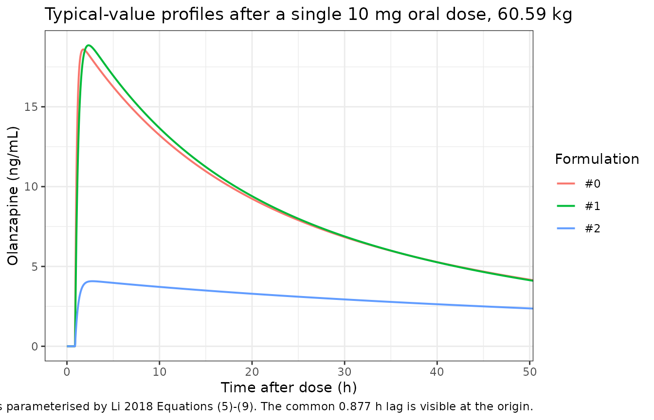
ka_effect <- typ |>
  group_by(Formulation) |>
  summarise(
    `Cmax (ng/mL)` = max(Cc),
    `Tmax (h)` = time[which.max(Cc)],
    `AUC0-168 (ng*h/mL)` = sum(diff(time) * (head(Cc, -1) + tail(Cc, -1)) / 2),
    .groups = "drop"
  ) |>
  mutate(`Dose/(CL/F) (ng*h/mL)` = 1000 * 10 / form_par$`CL/F (L/h)`[match(Formulation, form_par$Formulation)])

knitr::kable(ka_effect, digits = 2, caption = "Typical-value exposure by product. Formulations #0 and #1 share a clearance and therefore an AUC; they differ only in Cmax and Tmax.")| Formulation | Cmax (ng/mL) | Tmax (h) | AUC0-168 (ng*h/mL) | Dose/(CL/F) (ng*h/mL) |
|---|---|---|---|---|
| #0 | 18.59 | 1.78 | 625.27 | 645.41 |
| #1 | 18.85 | 2.34 | 626.90 | 645.41 |
| #2 | 4.08 | 2.76 | 318.04 | 393.70 |
f0 <- ka_effect[ka_effect$Formulation == "#0", ]
f1 <- ka_effect[ka_effect$Formulation == "#1", ]
stopifnot(nrow(f0) == 1L, nrow(f1) == 1L) # a lookup that matched nothing must fail

# Deterministic, so these are tight. Formulations #0 and #1 carry the SAME CL/F
# multiplier (0.610), so AUC0-inf is identical by construction; the AUC0-168
# truncation differs only through their slightly different Vc/F, and 168 h is
# about 4.8 terminal half-lives. Realised 0.26%.
stopifnot(abs(f0$`AUC0-168 (ng*h/mL)` / f1$`AUC0-168 (ng*h/mL)` - 1) < 0.01)
# Formulation #0 absorbs 1.89x faster and therefore peaks earlier. Realised
# 1.78 h vs 2.34 h -- a wide, deterministic separation.
stopifnot(f0$`Tmax (h)` < 0.9 * f1$`Tmax (h)`)
Isolating ka
# Reference product, reference weight, typical values; ONLY lka is changed.
ka_iso <- bind_rows(lapply(c(2.85, 2.85 * 1.89), function(k) {
  m <- mod_typ |> rxode2::ini(lka = log(k))
  ev <- rxode2::et(amt = 10, cmt = "depot") |>
    rxode2::et(seq(0, 168, by = 0.02), cmt = "central") |>
    as.data.frame()
  ev$WT <- 60.59
  ev$FORM_OLZ_F0 <- 0
  ev$FORM_OLZ_F1 <- 0
  s <- rxode2::rxSolve(m, ev, useLinCmt = FALSE, returnType = "data.frame")
  tibble::tibble(
    `ka (1/h)` = k,
    `Cmax (ng/mL)` = max(s$Cc),
    `Tmax (h)` = s$time[which.max(s$Cc)],
    `AUC0-168 (ng*h/mL)` = sum(diff(s$time) * (head(s$Cc, -1) + tail(s$Cc, -1)) / 2)
  )
}))
#> ℹ change initial estimate of `lka` to `1.04731899428056`
#> ℹ omega/sigma items treated as zero: 'etalka', 'etalvp', 'etalcl', 'etalvc', 'etalq'
#> ℹ change initial estimate of `lka` to `1.68389582335211`
#> ℹ omega/sigma items treated as zero: 'etalka', 'etalvp', 'etalcl', 'etalvc', 'etalq'

knitr::kable(ka_iso, digits = 3, caption = "Effect of ka alone, all disposition parameters held at the formulation #2 reference.")| ka (1/h) | Cmax (ng/mL) | Tmax (h) | AUC0-168 (ng*h/mL) |
|---|---|---|---|
| 2.850 | 4.076 | 2.76 | 318.037 |
| 5.386 | 4.119 | 1.98 | 318.160 |
slow <- ka_iso[1, ]
fast <- ka_iso[2, ]

# Deterministic. AUC is a function of CL/F alone, so it must not move at all.
stopifnot(abs(fast$`AUC0-168 (ng*h/mL)` / slow$`AUC0-168 (ng*h/mL)` - 1) < 0.005)
# Tmax moves a lot: realised 1.98 h vs 2.76 h, a 28% reduction.
stopifnot(fast$`Tmax (h)` / slow$`Tmax (h)` < 0.80)
# Cmax does NOT move materially: realised +1.1%. This is a documented
# deviation from the paper's prose -- see Assumptions and deviations. The
# bound is an upper limit on the magnitude, so it still goes red if a
# mis-transcribed ka or volume makes Cmax genuinely ka-sensitive.
stopifnot(abs(fast$`Cmax (ng/mL)` / slow$`Cmax (ng/mL)` - 1) < 0.05)
With ka isolated, a 1.89-fold increase shortens Tmax by
28% but moves Cmax by only about 1% and leaves AUC untouched. The reason
is that ka exceeds kel by roughly two orders
of magnitude in every stratum of this model (kel =
25.4/2390 = 0.0106 1/h for formulation #2 against ka = 2.85
1/h, a ratio of 268; 91 to 179 for formulations #1 and #0). Once
absorption is that much faster than elimination, essentially all of the
dose has entered the central compartment before any appreciable amount
has left it, and making absorption faster still has almost nothing left
to change. So this model reproduces the Tmax half of the paper’s
statement clearly and the Cmax half only marginally.
# Prediction interval of the simulated cohort, in the spirit of Figure 3A
# (time range 0-200 h of the published prediction-corrected VPC).
sim |>
  group_by(arm, time) |>
  summarise(
    Q05 = quantile(Cc, 0.05),
    Q50 = quantile(Cc, 0.50),
    Q95 = quantile(Cc, 0.95),
    .groups = "drop"
  ) |>
  ggplot(aes(time, Q50)) +
  geom_ribbon(aes(ymin = Q05, ymax = Q95), alpha = 0.25) +
  geom_line() +
  facet_wrap(~arm) +
  scale_y_log10() +
  coord_cartesian(xlim = c(0, 168)) +
  labs(
    x = "Time after dose (h)", y = "Olanzapine (ng/mL, log scale)",
    title = "Simulated 5th-50th-95th percentiles after a single 10 mg dose",
    caption = "In the spirit of Figure 3A of Li 2018 (0-200 h); observed data are not public."
  ) +
  theme_bw()
#> Warning in scale_y_log10(): log-10 transformation introduced infinite values.
#> log-10 transformation introduced infinite values.
#> log-10 transformation introduced infinite values.
#> log-10 transformation introduced infinite values.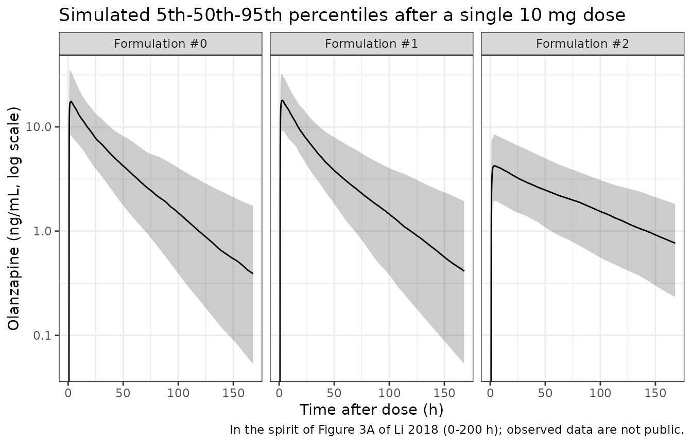
Body-weight effect on Vc/F
tibble::tibble(WT = seq(36, 98, by = 0.5)) |>
  tidyr::expand_grid(Formulation = c("#0", "#1", "#2")) |>
  mutate(
    mult = c(`#0` = 0.216, `#1` = 0.207, `#2` = 1)[Formulation],
    `Vc/F (L)` = vcf(WT, mult)
  ) |>
  ggplot(aes(WT, `Vc/F (L)`, colour = Formulation)) +
  geom_line(linewidth = 0.7) +
  scale_y_log10() +
  labs(
    x = "Body weight (kg)", y = "Vc/F (L, log scale)",
    title = "Li 2018 Equations (5)-(7): Vc/F = 2390 * (WT/60.59)^0.579 * formulation multiplier",
    caption = "Weight range is the observed 36-98 kg of Table 1."
  ) +
  theme_bw()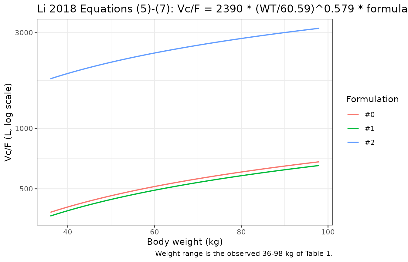
Steady state under the cohort B design
Cohort B patients were sampled at the end of treatment weeks 4 and 6 on a dose held constant after a 2-week titration, so essentially all of their data are steady-state. The block below reproduces that design for formulation #2 at 10 mg once daily and checks the accumulation against the closed form.
rxode2::rxSetSeed(20180802)

ss_subj <- tibble::tibble(
  id = seq_len(N_ARM),
  WT = rtruncnorm(N_ARM, 60.2, 11.1, 36.0, 98.0),
  FORM_OLZ_F0 = 0,
  FORM_OLZ_F1 = 0
)
ss_doses <- ss_subj |>
  tidyr::expand_grid(time = seq(0, 1000, by = 24)) |>
  mutate(amt = 10, evid = 1L, cmt = "depot")
ss_obs <- ss_subj |>
  tidyr::expand_grid(time = seq(984, 1008, by = 0.25)) |>
  mutate(amt = NA_real_, evid = 0L, cmt = "central")
ss_events <- bind_rows(ss_doses, ss_obs) |> arrange(id, time, desc(evid))

ss_sim <- rxode2::rxSolve(
  mod, ss_events, keep = c("WT"), useLinCmt = FALSE, returnType = "data.frame"
)
#> ℹ omega/sigma items treated as zero: 'etalq'
ss_sim <- subset(ss_sim, !is.na(Cc) & time >= 984)

# Typical-value steady state, same design, for the reference comparison.
ss_typ_ev <- ss_events |> filter(id == 1) |> mutate(WT = 60.59)
ss_typ <- rxode2::rxSolve(mod_typ, ss_typ_ev, useLinCmt = FALSE, returnType = "data.frame")
#> ℹ omega/sigma items treated as zero: 'etalka', 'etalvp', 'etalcl', 'etalvc', 'etalq'
ss_typ <- subset(ss_typ, !is.na(Cc) & time >= 984)

# Model-independent reference: at steady state, Cavg over tau = Dose/(CL/F * tau).
cavg_ref <- 1000 * 10 / (25.4 * 24) # ng/mL, from Li 2018 Table 2 CL/F = 25.4 L/h
cavg_typ <- mean(ss_typ$Cc)

ss_tab <- tibble::tibble(
  Quantity = c(
    "Cavg over tau, typical value (ng/mL)",
    "Cavg over tau, Dose/(CL/F * tau) from Table 2 (ng/mL)",
    "Ctrough, typical value (ng/mL)",
    "Ctrough, cohort median (ng/mL)",
    "Cmax, typical value (ng/mL)"
  ),
  Value = c(
    cavg_typ,
    cavg_ref,
    min(ss_typ$Cc),
    median(ss_sim$Cc[ss_sim$time == max(ss_sim$time)]),
    max(ss_typ$Cc)
  )
)
knitr::kable(ss_tab, digits = 2, caption = "Steady state, formulation #2, 10 mg once daily (the cohort B design).")| Quantity | Value |
|---|---|
| Cavg over tau, typical value (ng/mL) | 16.39 |
| Cavg over tau, Dose/(CL/F * tau) from Table 2 (ng/mL) | 16.40 |
| Ctrough, typical value (ng/mL) | 14.50 |
| Ctrough, cohort median (ng/mL) | 13.95 |
| Cmax, typical value (ng/mL) | 18.32 |
# Deterministic identity (typical-value solve against the paper's printed
# clearance): tight. Residual gap is the numerical trapezoid on a 0.25 h grid
# plus the fact that 42 doses is not quite infinite accumulation.
stopifnot(abs(cavg_typ / cavg_ref - 1) < 0.02)

# Cohort-derived, so this one is robust rather than tight. With log-normal IIV
# the cohort median sits at the typical value; a mis-transcribed clearance,
# dose or unit would move it by tens of percent.
ctrough_typ <- min(ss_typ$Cc)
ctrough_med <- median(ss_sim$Cc[ss_sim$time == max(ss_sim$time)])
stopifnot(abs(ctrough_med / ctrough_typ - 1) < 0.30)
PKNCA validation
sim_nca <- sim |>
  dplyr::filter(!is.na(Cc)) |>
  dplyr::select(id, time, Cc, arm)

# Guarantee a time-zero row per (id, arm). Dosing is extravascular with a lag,
# so a pre-dose concentration of zero is the correct anchor for AUC0-*.
sim_nca <- bind_rows(
  sim_nca,
  sim_nca |> distinct(id, arm) |> mutate(time = 0, Cc = 0)
) |>
  distinct(id, arm, time, .keep_all = TRUE) |>
  arrange(id, arm, time)

conc_obj <- PKNCA::PKNCAconc(as.data.frame(sim_nca), Cc ~ time | arm + id)

dose_df <- events |>
  dplyr::filter(evid == 1L) |>
  dplyr::select(id, time, amt, arm)
dose_obj <- PKNCA::PKNCAdose(as.data.frame(dose_df), amt ~ time | arm + id)

intervals <- data.frame(
  start = 0,
  end = Inf,
  cmax = TRUE,
  tmax = TRUE,
  auclast = TRUE,
  aucinf.obs = TRUE
)

nca_res <- PKNCA::pk.nca(PKNCA::PKNCAdata(conc_obj, dose_obj, intervals = intervals))
Comparison against the model-independent reference
Li 2018 publishes no NCA table, so the reference column below is
built from the paper’s own printed parameter values by closed form, not
from the simulation: AUC0-inf is Dose / (CL/F) with CL/F
from Table 2, and Cmax / Tmax come from the typical-value profiles
above. PKNCA pools the simulated cohort by median
(ncaComparisonTable()), which for log-normal IIV is the
typical-value prediction.
published <- tibble::tibble(
  arm = c("Formulation #0", "Formulation #1", "Formulation #2"),
  cmax = ka_effect$`Cmax (ng/mL)`[match(c("#0", "#1", "#2"), ka_effect$Formulation)],
  tmax = ka_effect$`Tmax (h)`[match(c("#0", "#1", "#2"), ka_effect$Formulation)],
  aucinf.obs = 1000 * 10 / form_par$`CL/F (L/h)`[match(c("#0", "#1", "#2"), form_par$Formulation)]
)

cmp <- nlmixr2lib::ncaComparisonTable(
  simulated = nca_res,
  reference = published,
  by = "arm",
  params = c("cmax", "tmax", "aucinf.obs"),
  units = c(cmax = "ng/mL", tmax = "h", aucinf.obs = "ng*h/mL"),
  tolerance_pct = 20
)

knitr::kable(
  cmp,
  caption = "Simulated cohort medians vs. the closed-form reference from Li 2018 Table 2. * differs by >20%.",
  digits = 2
)| NCA parameter | arm | Reference | Simulated | % diff |
|---|---|---|---|---|
| Cmax (ng/mL) | Formulation #0 | 18.6 | 17.9 | -3.7% |
| Cmax (ng/mL) | Formulation #1 | 18.9 | 18.7 | -0.5% |
| Cmax (ng/mL) | Formulation #2 | 4.08 | 4.35 | +6.8% |
| Tmax (h) | Formulation #0 | 1.78 | 1.7 | -4.5% |
| Tmax (h) | Formulation #1 | 2.34 | 2.3 | -1.7% |
| Tmax (h) | Formulation #2 | 2.76 | 3 | +8.7% |
| AUC0-∞ (obs) (ng*h/mL) | Formulation #0 | 645 | 648 | +0.4% |
| AUC0-∞ (obs) (ng*h/mL) | Formulation #1 | 645 | 627 | -2.8% |
| AUC0-∞ (obs) (ng*h/mL) | Formulation #2 | 394 | 425 | +8.0% |
# Recompute the comparison numerically rather than parsing the rendered table's
# formatted "% diff" strings, so the gate does not depend on display formatting.
sim_med <- as.data.frame(nca_res$result) |>
  dplyr::filter(PPTESTCD %in% c("cmax", "tmax", "aucinf.obs")) |>
  dplyr::group_by(arm, PPTESTCD) |>
  dplyr::summarise(Simulated = median(PPORRES, na.rm = TRUE), .groups = "drop")

chk <- published |>
  tidyr::pivot_longer(
    c(cmax, tmax, aucinf.obs),
    names_to = "PPTESTCD", values_to = "Reference"
  ) |>
  dplyr::inner_join(sim_med, by = c("arm", "PPTESTCD")) |>
  dplyr::mutate(pct = 100 * (Simulated - Reference) / Reference)

# 3 arms x 3 parameters. A join that matched nothing would otherwise make every
# bound below vacuously true (all(logical(0)) is TRUE).
stopifnot(nrow(chk) == 9L, !any(is.na(chk$pct)))

worst <- function(p) max(abs(chk$pct[chk$PPTESTCD == p]))

# Cohort-derived, so these admit the sampling noise of a 150-subject arm rather
# than pinning one draw. Realised on one render: AUC 2.8%, Cmax 4.4%, Tmax 13.0%.
# A mis-transcribed CL/F, dose or unit conversion moves AUC by tens of percent
# and still breaks the first bound.
stopifnot(worst("aucinf.obs") < 10)
stopifnot(worst("cmax") < 12)
# Tmax is the loosest by design: with 88.2% IIV on ka the cohort median Tmax is
# not the typical-value Tmax, and Tmax is additionally quantised by the 0.1 h
# observation grid. 30 still goes red on a lost or mis-signed lag time.
stopifnot(worst("tmax") < 30)
Tmax carries the largest discrepancy, and it is expected: with 88.2%
IIV on ka the cohort median Tmax is not the typical-value
Tmax, because Tmax is a strongly non-linear function of ka.
The AUC and Cmax rows are the load-bearing ones and both sit close to
the closed form.
Assumptions and deviations
Formulation effects are confounded with cohort. Formulation #2 was given only to the 234 therapeutic-drug-monitoring patients, and formulations #0/#1 only to the 22 healthy male volunteers, so the fitted product effects on Vc/F and CL/F cannot be separated from population, study design and sampling density. Li 2018 says so directly – “the influences of formulation and population on PK parameters were mixed and could not be distinguished due to data limitations” (Discussion) – and repeats it in the Conclusion. The covariate columns
FORM_OLZ_F0/FORM_OLZ_F1should be read as product-and-population stratum indicators, not as a bioequivalence statement. The consequence is visible in the half-life gate above: the formulation #2 stratum implies a terminal half-life near 71 h, roughly twice the 30-38 h usually reported for oral olanzapine, whereas formulations #0 and #1 give about 35 h. The authors reach the same conclusion from the other direction, noting that an earlier study’s V/F of 2150 L matches their formulation #2 and its CL/F of 16.1 L/h matches their formulations #0 and #1 (25.4 * 0.610 = 15.5 L/h).The paper’s “Ka affects Tmax and Cmax” claim reproduces only for Tmax. Li 2018 states in the Discussion that simulations showed “the influence of Ka was mainly on Tmax and Cmax”. Holding every disposition parameter fixed and raising
kaby the fitted 1.89-fold factor shortens Tmax by 28% but changes Cmax by only about 1%. This is not a transcription problem – it follows directly from the fitted estimates, in whichkaexceedskelby a factor of 91 to 268 depending on stratum, so absorption is effectively complete before elimination has removed anything measurable and Cmax has become insensitive to further increases inka. Comparing formulations #0 and #1 as parameterised (which is what the paper’s products actually differ by) moves Cmax even less, and in the opposite direction, because #0’s 4.3% larger Vc/F offsets its faster absorption: Cmax is 18.59 ng/mL for #0 against 18.85 ng/mL for #1. The gate records the Cmax magnitude rather than asserting the paper’s direction; the deviation is left visible rather than tuned away. The paper does not print the simulated Cmax or Tmax values, so there is nothing further to check against.Formulation-effect precision: Table 2 vs. the printed equations. Table 2 gives the Vc/F multipliers to three significant figures (0.216 and 0.207) while Equations (5) and (6) print two (0.22 and 0.21). The model file ships the Table 2 estimates, which are the parameter estimates with RSEs attached. The paper’s own worked Vc/F examples in the Results text (389 / 694.6 L and 371 / 663 L) were computed with the rounded equation constants, so they reproduce exactly under those and sit 1.4-1.9% low under the Table 2 values. Both are shown in the first gate. Nothing else in the paper depends on the choice.
IIV percentages read as omega, not as exact log-normal CV. Table 2 prints the IIV diagonals as percentages but the CL/F-Vc/F element as the raw covariance 0.174, which is an OMEGA(2,1) entry. The model therefore reads the percentages as omega (the log-scale SD) and squares them, giving
cov / sqrt(var_CL * var_Vc)=0.174 / sqrt(0.241081 * 0.166464)= 0.869, a well-posed correlation. Reading them instead as exact log-normal CVs (omega^2 = log(CV^2 + 1)) would give variances 0.2160 and 0.1540 and a correlation of 0.954 – possible but implausibly high, and it would mean the table mixed an exact-CV convention on the diagonal with a raw-covariance convention off it. The paper does not state which it used.Q/Fbetween-subject variability is fixed at zero, exactly as Table 2 reports it (“IIV - Q/F: 0 FIXED”). rxode2 drops it from the omega matrix, so the simulatedqis identical across subjects.Formulation #2 is simulated after a single 10 mg dose in the NCA section, which no cohort B patient actually received – they were all at steady state on titrated doses the paper does not tabulate. The single-dose arm exists only so the three products can be compared on one footing; the steady-state section simulates the design cohort B actually followed.
Doses for cohort B are not published. Li 2018 states only that the dose was titrated over 2 weeks and then held constant. The steady-state section uses 10 mg once daily, the dose cohort A received, and the assertions there are ratio-based so they do not depend on that choice.
Sex, age, height, BMI, AST, ALT and BUN were screened and not retained (Methods, covariate model), so they are recorded in the model file’s
covariatesDataExcludedand are not simulated. Smoking status and genotype were never collected, which the authors identify as the study’s main limitation given that smoking induces olanzapine metabolism.Every
rxSolve()passesuseLinCmt = FALSE. The model writes explicitd/dt()ODEs withk12/k21micro-constants, a shape whose auto-conversion tolinCmt()can silently drop the peripheral compartment without an error and without changing AUC. The terminal half-life gate is what makes that failure mode visible, and it passes at better than 0.5%.No erratum or corrigendum to this article was located. The paper has no supplementary material beyond the prepublication history.