Model and source
- Citation: Gaspar F, Terrier J, Favre S, Gosselin P, Fontana P, Daali Y, Lenoir C, Samer CF, Rollason V, Reny JL, Csajka C, Guidi M. Population pharmacokinetics of apixaban in a real-life hospitalized population from the OptimAT study. CPT Pharmacometrics Syst Pharmacol. 2023;12(10):1541-1552. doi:10.1002/psp4.13032.
- Description: Two-compartment population pharmacokinetic model with first-order absorption and an absorption lag time for oral apixaban in a real-life cohort of hospitalized, mostly elderly patients from the OptimAT study (Gaspar 2023). Apparent oral clearance CL/F = 3.2 L/h at a Cockcroft-Gault creatinine clearance of 100 mL/min and a P-glycoprotein phenotyping index (fexofenadine AUC from 2 to 6 h) of 205 mg*h/L, scaled by the power terms (CRCL/100)^0.47 and (AUC_FEXO/205)^-0.17. Renal function and P-gp phenotypic activity together explained 58% of the between-patient variance in clearance (41% and 17%, respectively). Apparent central and peripheral volumes are 27 L and 51 L, apparent intercompartmental clearance 16 L/h, absorption rate constant 0.82 1/h and lag time 0.16 h. Variability is carried as interoccasion variability on clearance (30% CV, one occasion per hospitalization) rather than interindividual variability, with interindividual variability on lag time (108% CV), absorption rate (58% CV), intercompartmental clearance (65% CV) and peripheral volume (88% CV); interindividual variability on the central volume was tested and not retained. Residual variability is proportional (8.4% CV). Neither CYP3A4/5 phenotypic activity nor any demographic or laboratory covariate was retained. Parameter values are taken from the publication’s Table 2 (Final model column) and the final-model equation printed in the Table 2 note.
- Article: https://doi.org/10.1002/psp4.13032
Gaspar 2023 is, in the authors’ words, the first population PK model of apixaban built on data collected in a real-world population of hospitalized patients rather than in a clinical trial. Its practical purpose is pre-procedural: to predict how long after the last dose a patient’s apixaban concentration falls below the 50 ng/mL threshold that current consensus regards as safe for an invasive procedure, and to show that the standardized interruption schedules in the PAUSE study are too short for patients with impaired renal function or reduced P-glycoprotein activity.
Population
The model was fitted to 825 apixaban concentrations from 100 hospitalized patients enrolled in the OptimAT study (NCT03477331), a single-centre prospective observational study at the Geneva University Hospitals running from January 2018 to November 2019 (Gaspar 2023 Methods, “Study population”). Each participant underwent one day of multiple finger-prick dried-blood-spot sampling after their morning dose, scheduled predose and at 0.5, 1, 2, 3, 4, 6 and 8 h, giving a median of 8 samples per patient (range 7-8). Six patients were hospitalized twice, so the 100 patients contributed 106 occasions.
Per Table 1, the cohort is elderly and renally impaired: median age 77 years (range 51-94), median body weight 75 kg (range 44-126), 42% female, and a median Cockcroft-Gault creatinine clearance of only 57.2 mL/min (range 23-136). Apixaban was prescribed for atrial fibrillation in 89% of patients and for venous thromboembolism in 11%, at 2.5 mg b.i.d. (n = 40), 5 mg b.i.d. (n = 56) or 10 mg b.i.d. (n = 4). Phenotyping with the Geneva cocktail classified 47% of the cohort as P-glycoprotein poor metabolizers, 51% as normal and 2% as ultra-rapid; the corresponding CYP3A4/5 split was 19% / 78% / 3%. An independent cohort of 63 patients from the DAPHNE study (NCT03112525) was used for external validation, where the model showed a mean prediction error of 0% (95% CI -1% to 1%) and a precision of 11%.
Apixaban was quantified in whole blood by LC-MS/MS and converted to a
plasma concentration with the Foerster relationship
Conc_plasma = Conc_DBS * 1.46 + 13.84, so the model
predicts plasma concentrations.
The same information is available programmatically via the model’s
population metadata
(readModelDb("Gaspar_2023_apixaban")()$population).
Source trace
The per-parameter origin is recorded as an in-file comment next to
each ini() entry in
inst/modeldb/specificDrugs/Gaspar_2023_apixaban.R. The
table below collects them in one place for review. All values come from
Table 2, column “Final model Estimate (RSE %)”, except where noted.
| Equation / parameter | Value | Source location |
|---|---|---|
ltlag (Tlag) |
0.16 h | Table 2 (RSE 19%; bootstrap 0.18 [0.07-0.28]) |
lka (ka) |
0.82 1/h | Table 2 (RSE 11%; bootstrap 0.92 [0.54-1.87]) |
lcl (CL/F) |
3.2 L/h | Table 2 (RSE 6%; bootstrap 3.1 [2.4-3.6]) |
lvc (Vc/F) |
27 L | Table 2 (RSE 8%; bootstrap 29 [18-44]) |
lq (Q/F) |
16 L/h | Table 2 (RSE 12%; bootstrap 14 [8.0-27]) |
lvp (Vp/F) |
51 L | Table 2 (RSE 12%; bootstrap 56 [25-118]) |
e_crcl_cl (beta_CLcr) |
0.47 | Table 2 (RSE 19%; bootstrap 0.47 [0.22-0.74]) |
e_auc_fexo_cl (beta_P-gp) |
-0.17 | Table 2 (RSE 32%; bootstrap -0.21 [-0.44 to -0.05]) |
| CRCL centring constant | 100 mL/min | Methods “Covariate model” and the Table 2 note equation |
| AUC_FEXO centring constant | 205 mg*h/L | Table 2 note equation |
etaltlag |
108% CV -> 0.77307 | Table 2 “IIV Tlag (CV%)”; omega^2 = log(CV^2 + 1) |
etalka |
58% CV -> 0.28998 | Table 2 “IIV ka (CV%)” |
etalq |
65% CV -> 0.35242 | Table 2 “IIV Q (CV%)” |
etalvp |
88% CV -> 0.57346 | Table 2 “IIV Vp (CV%)” |
etaiov_cl_1/2 |
30% CV -> 0.08618 | Table 2 “IOV CL (CV%)”; one occasion per hospitalization (Methods) |
propSd |
0.084 | Table 2 “Proportional error model (CV%)” = 8.4% |
Covariate model form
(Cov/Cov_weight)^beta * exp(eta)
|
n/a | Methods “Covariate model”, Equation 1 |
| Final clearance equation | n/a | Table 2 note:
CL_occ,i = CL * (CLcr/100)^beta_CLcr * (AUC2-6/205)^beta_PgP * exp(IOV_CL,occ,i)
|
| Two-compartment structure, first-order absorption + lag | n/a | Results “Base model” |
| No IIV on CL (replaced by IOV); no IIV on Vc | n/a | Results “Base model” (dOFV = -110 for IOV; dOFV = 1.7, p > 0.05 for IIV on Vc) |
| Proportional residual error | n/a | Results “Base model” |
| Phenotype-category P-gp AUC2-6 means | 285.5 / 100.1 / 50.4 mg*h/L | Methods “Phenotyping” and Table 3 footnote |
| CKD stage CLcr bands | see below | Methods “Model-based simulations” |
| 50 ng/mL pre-procedural target | 50 ng/mL | Methods “Model-based simulations”; Table 3 |
| 230 ng/mL bleeding-risk threshold | 230 ng/mL | Methods “Model-based simulations”; Figure 2 |
Deterministic checks against the paper’s own derived quantities
Before simulating a cohort, three quantities that follow deterministically from the Table 2 parameters can be checked against numbers the paper prints elsewhere. These are pure algebra on the transcribed values, so they are the sharpest available test that the transcription is right, and they are gated tightly.
ui <- rxode2::rxode(readModelDb("Gaspar_2023_apixaban"))
#> ℹ parameter labels from comments will be replaced by 'label()'
#> Warning: some etas defaulted to non-mu referenced, possible parsing error: etaiov_cl_1, etaiov_cl_2
#> as a work-around try putting the mu-referenced expression on a simple line
th <- setNames(ui$theta, names(ui$theta))

cl_typ <- exp(th[["lcl"]])
vc     <- exp(th[["lvc"]])
q      <- exp(th[["lq"]])
vp     <- exp(th[["lvp"]])

# Typical clearance for the reference patient the paper's Results section uses:
# a P-gp NORMAL metabolizer (AUC2-6 = 100.1 mg*h/L) with normal renal function
# (CLcr = 100 mL/min). Note that this is NOT the bare 3.2 L/h of Table 2: the
# equation centres the P-gp term at 205 mg*h/L, not at the NM mean.
cl_nm <- cl_typ * (100 / 100)^th[["e_crcl_cl"]] *
  (100.1 / 205)^th[["e_auc_fexo_cl"]]

# Two-compartment macro rate constants.
twocmt_halflives <- function(cl, vc, q, vp) {
  k10 <- cl / vc
  k12 <- q / vc
  k21 <- q / vp
  a <- k10 + k12 + k21
  b <- k10 * k21
  lam1 <- (a + sqrt(a^2 - 4 * b)) / 2
  lam2 <- (a - sqrt(a^2 - 4 * b)) / 2
  c(alpha = log(2) / lam1, beta = log(2) / lam2)
}
hl <- twocmt_halflives(cl_nm, vc, q, vp)

# Covariate effect sizes relative to a P-gp normal metabolizer.
pgp_ratio <- function(auc) (auc / 205)^th[["e_auc_fexo_cl"]] / (100.1 / 205)^th[["e_auc_fexo_cl"]]

det <- tibble::tibble(
  Quantity = c(
    "Typical CL/F, P-gp NM, CLcr 100 (L/h)",
    "Distribution half-life t1/2 alpha (h)",
    "Terminal half-life t1/2 beta (h)",
    "Total volume of distribution Vc + Vp (L)",
    "CL/F ratio, P-gp PM vs NM",
    "CL/F ratio, P-gp UM vs NM"
  ),
  Model = c(cl_nm, hl[["alpha"]], hl[["beta"]], vc + vp,
            pgp_ratio(285.5), pgp_ratio(50.4)),
  Published = c(NA, 0.70, 17, 78, 0.84, 1.12),
  `Source` = c(
    "derived",
    "Results 'Covariate analyses': 0.70 h (alpha)",
    "Results 'Covariate analyses': 17 h (beta)",
    "Discussion: 'The total volume of distribution of 78 L'",
    "Results: CL 'reduced by 16%' in P-gp PM",
    "Results: CL 'increased by 12%' in P-gp UM"
  )
)
knitr::kable(det, digits = 3,
caption = "Quantities derived algebraically from the Table 2 parameters, against the values Gaspar 2023 reports in prose.")| Quantity | Model | Published | Source |
|---|---|---|---|
| Typical CL/F, P-gp NM, CLcr 100 (L/h) | 3.615 | NA | derived |
| Distribution half-life t1/2 alpha (h) | 0.694 | 0.70 | Results ‘Covariate analyses’: 0.70 h (alpha) |
| Terminal half-life t1/2 beta (h) | 16.472 | 17.00 | Results ‘Covariate analyses’: 17 h (beta) |
| Total volume of distribution Vc + Vp (L) | 78.000 | 78.00 | Discussion: ‘The total volume of distribution of 78 L’ |
| CL/F ratio, P-gp PM vs NM | 0.837 | 0.84 | Results: CL ‘reduced by 16%’ in P-gp PM |
| CL/F ratio, P-gp UM vs NM | 1.124 | 1.12 | Results: CL ‘increased by 12%’ in P-gp UM |
stopifnot(
  # Deterministic algebra on transcribed constants -- no simulation, no cohort,
  # so these are gated to the paper's own reporting precision. A mis-transcribed
  # volume, clearance or exponent moves each of them by tens of percent.
  abs(hl[["alpha"]] - 0.70) < 0.05,
  abs(hl[["beta"]] - 17) < 1.5,
  abs((vc + vp) - 78) < 0.5,
  abs(pgp_ratio(285.5) - 0.84) < 0.01,
  abs(pgp_ratio(50.4) - 1.12) < 0.01
)
The half-lives, the total volume of distribution and both
P-glycoprotein effect sizes reproduce to the precision the paper reports
them. This also confirms the reading of the centring constant 205 mg*h/L
in the Table 2 note equation: had CL = 3.2 L/h instead been
the clearance of a P-gp normal metabolizer, the terminal
half-life would come out at 18.4 h rather than the 16.5 h that rounds to
the published 17 h, and the alpha half-life would be unchanged, so the
beta half-life is what discriminates the two readings.
One published derived quantity is not reproduced; see “Assumptions and deviations” below.
Virtual cohort
Original observed data are not publicly available. The cohort below follows the paper’s own simulation design (Methods, “Model-based simulations”): 5 chronic kidney disease stages crossed with 3 P-glycoprotein phenotypes, with a uniform distribution assumed over each covariate’s range.
# set.seed() seeds R's RNG. It does NOT seed rxode2's simulation RNG, and
# rxode2's streams are partitioned PER SOLVER THREAD, so this cohort is
# reproducible on this machine and different on a machine with a different
# thread count. Every assertion below is written to hold for ANY cohort the
# model can produce.
set.seed(20231001)

# 50 per arm across 15 arms (750 subjects). Sized against the render time:
# the vignette must stay well under 5 minutes even when rendered in
# parallel with other vignettes, where CPU contention multiplies
# wall-clock time. Measured single-threaded here at
# 40 / 75 / 100 per arm: 54 / 168 / 203 s (the PKNCA step scales worse than
# linearly), so this sits at roughly 80 s with ample headroom. The only gates
# that depend on cohort size are the Table 3 medians, which are checked on
# robust statistics rather than extremes.
n_per_arm <- 50L

# CKD bands per Methods "Model-based simulations". Stage 1 is defined as
# CLcr > 90 mL/min with no upper bound, so it is capped at the observed cohort
# maximum of 136 mL/min (Table 1). Stage 5 is defined as CLcr < 15 mL/min and
# is capped below at 5 mL/min; both stage 4 and stage 5 extend below the
# observed cohort minimum of 23 mL/min and are therefore extrapolation, which
# the paper also performs.
ckd_bands <- tibble::tribble(
  ~ckd,      ~crcl_lo, ~crcl_hi,
  "Stage 1",       90,      136,
  "Stage 2",       60,       89,
  "Stage 3",       30,       59,
  "Stage 4",       15,       29,
  "Stage 5",        5,       15
)

# P-gp phenotype bands. Methods "Phenotyping" gives category mean +/- SD for the
# fexofenadine AUC(2-6 h) index; Methods "Model-based simulations" says a
# uniform distribution over the studied range was assumed, which is read here as
# uniform over mean +/- SD. See "Assumptions and deviations".
pgp_bands <- tibble::tribble(
  ~pgp,  ~auc_mean, ~auc_sd,
  "PM",      285.5,    67.1,
  "NM",      100.1,    47.5,
  "UM",       50.4,    15.3
) |>
  mutate(auc_lo = auc_mean - auc_sd, auc_hi = auc_mean + auc_sd)

arms <- tidyr::crossing(ckd_bands, pgp_bands) |>
  mutate(arm = paste(ckd, pgp)) |>
  arrange(ckd, factor(pgp, levels = c("PM", "NM", "UM")))

# Steady-state 5 mg b.i.d., delivered as a single steady-state dose record
# (`ss = 1`, `ii = 12`) at t = 0 rather than as a 20-dose burn-in. Time 0 is
# therefore the last drug intake, which is exactly the time origin Gaspar 2023
# Figure 3 and Table 3 use. This was verified against an explicit 20-dose q12h
# solve: the two agree to a relative 7e-5, and it removes 228 h of burn-in
# integration per subject from the render.
#
# The model is strictly linear, so the 2.5 and 10 mg columns of Table 3 are
# recovered later by rescaling the concentration threshold rather than by
# re-simulating.
tau <- 12

# Observation grid, graded: fine over the dosing interval (for Cmin / Cmax /
# AUC at steady state), then progressively coarser out to 240 h, where Table 3
# censors. The published medians span 6-149 h, so the grid resolution is kept
# well under 5% of the crossing time throughout.
obs_times <- sort(unique(c(
  seq(0, 12, by = 0.25),
  seq(12, 48, by = 1),
  seq(48, 120, by = 3),
  seq(120, 240, by = 6)
)))

make_arm <- function(n, arm, crcl_lo, crcl_hi, auc_lo, auc_hi, id_offset) {
  subj <- tibble::tibble(
    id       = id_offset + seq_len(n),
    arm      = arm,
    CRCL     = runif(n, crcl_lo, crcl_hi),
    AUC_FEXO = runif(n, auc_lo, auc_hi),
    # One hospitalization per simulated patient, so the first IOV eta applies.
    OCC      = 1L
  )
  doses <- subj |>
    mutate(time = 0, amt = 5, evid = 1L, cmt = "depot", ss = 1L, ii = tau)
  obs <- subj |>
    tidyr::crossing(time = obs_times) |>
    # Observations are placed on the ODE state `central`, never on the
    # algebraic observable `Cc`; rxode2 returns Cc as a column regardless.
    mutate(amt = NA_real_, evid = 0L, cmt = "central", ss = 0L, ii = 0)
  bind_rows(doses, obs) |> arrange(id, time, desc(evid))
}

events <- do.call(bind_rows, lapply(seq_len(nrow(arms)), function(i) {
  a <- arms[i, ]
  make_arm(n_per_arm, a$arm, a$crcl_lo, a$crcl_hi, a$auc_lo, a$auc_hi,
           id_offset = (i - 1L) * n_per_arm)
}))

# Disjoint IDs across arms are mandatory: rxSolve treats id as the subject key
# and would silently merge duplicates into one over-dosed subject.
stopifnot(!anyDuplicated(unique(events[, c("id", "time", "evid")])))
stopifnot(nrow(dplyr::distinct(events, id)) == n_per_arm * nrow(arms))
Simulation
mod <- readModelDb("Gaspar_2023_apixaban")
sim <- rxode2::rxSolve(mod, events = events,
                       keep = c("arm", "CRCL", "AUC_FEXO"),
                       # steady-state searches for long-half-life subjects exceed the default step budget
                       maxsteps = 1e6) |>
  as.data.frame()
#> ℹ parameter labels from comments will be replaced by 'label()'
#> Warning: some etas defaulted to non-mu referenced, possible parsing error: etaiov_cl_1, etaiov_cl_2
#> as a work-around try putting the mu-referenced expression on a simple line

# `Cc` is the individual prediction; it carries no residual error (the
# proportional error term is applied at the observation level, not here), which
# is what the paper's simulations of Cmin and stopping time use.
sim <- sim |>
  mutate(
    ckd  = sub("^(Stage \\d).*$", "\\1", arm),
    pgp  = sub("^Stage \\d ", "", arm),
    # Time 0 is the last drug intake, so time after dose is the time column.
    tad  = time
  )
stopifnot(all(!is.na(sim$Cc)), all(sim$Cc >= 0))
Replicate Figure 2: steady-state Cmin by CKD stage and P-gp activity
Figure 2 of Gaspar 2023 shows the distribution of the simulated steady-state minimum concentration for each CKD stage and P-gp phenotype, against the 5th-95th percentile band of Cmin reported by the manufacturer in atrial fibrillation (41-230 ng/mL for 5 mg b.i.d.) and the 230 ng/mL concentration associated with a 20% increased bleeding risk.
# Replicates Figure 2 of Gaspar 2023 (5 mg b.i.d. panel).
cmin_tbl <- sim |>
  filter(tad >= 0, tad <= 12) |>
  group_by(id, arm, ckd, pgp) |>
  summarise(cmin = min(Cc), .groups = "drop") |>
  mutate(pgp = factor(pgp, levels = c("PM", "NM", "UM")))

ggplot(cmin_tbl, aes(x = ckd, y = cmin, fill = pgp)) +
  annotate("rect", xmin = -Inf, xmax = Inf, ymin = 41, ymax = 230,
           alpha = 0.15, fill = "grey40") +
  geom_hline(yintercept = 230, linewidth = 0.6) +
  geom_boxplot(outlier.size = 0.5, position = position_dodge(width = 0.8)) +
  scale_y_log10() +
  labs(x = "Chronic kidney disease stage", y = "Steady-state Cmin (ng/mL)",
       fill = "P-gp activity",
       title = "Figure 2 - steady-state Cmin, apixaban 5 mg b.i.d.",
       caption = paste("Replicates Figure 2 of Gaspar 2023. Grey band: 41-230 ng/mL,",
                       "the manufacturer's 5th-95th percentile of Cmin in atrial",
                       "fibrillation. Black line: 230 ng/mL bleeding-risk threshold."))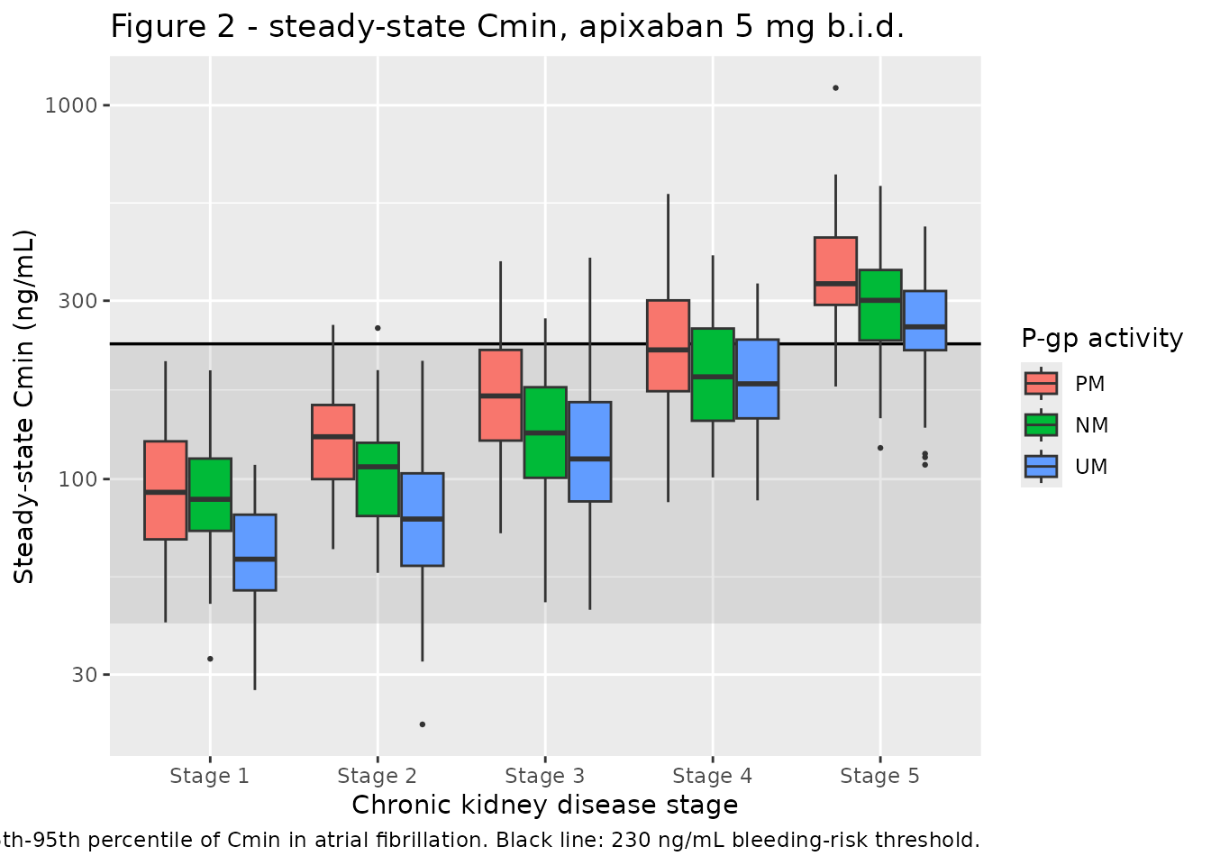
The paper makes three quantitative claims about this figure. Checking them on the medians of the cohort above would be checking a statistic with meaningful sampling noise at 50 subjects per arm, so they are instead evaluated on a typical-value (variability-suppressed) solve at each stratum’s midpoint covariates. That makes each number a deterministic property of the transcribed parameters, and the gates correspondingly sharp.
ckd_mid <- ckd_bands |> mutate(crcl = (crcl_lo + crcl_hi) / 2) |> select(ckd, crcl)
# Phenotype-category MEANS from Methods "Phenotyping", not the band midpoints.
pgp_mid <- pgp_bands |> select(pgp, auc = auc_mean)

grid <- tidyr::crossing(ckd_mid, pgp_mid) |> mutate(id = dplyr::row_number())

grid_ev <- bind_rows(
  grid |> mutate(time = 0, amt = 5, evid = 1L, cmt = "depot", ss = 1L, ii = tau),
  grid |> tidyr::crossing(time = seq(0, tau, by = 0.05)) |>
    mutate(amt = NA_real_, evid = 0L, cmt = "central", ss = 0L, ii = 0)
) |>
  mutate(CRCL = crcl, AUC_FEXO = auc, OCC = 1L) |>
  # Drop the lower-case staging columns before the solve: carrying both `crcl`
  # and `CRCL` through rxSolve collides on a case-insensitive name match.
  select(id, time, amt, evid, cmt, ss, ii, CRCL, AUC_FEXO, OCC, ckd, pgp) |>
  arrange(id, time, desc(evid))

typ_cmin <- rxode2::rxSolve(mod |> rxode2::zeroRe(), events = grid_ev,
                            keep = c("ckd", "pgp"),
                            # steady-state searches for long-half-life subjects exceed the default step budget
                            maxsteps = 1e6) |>
  as.data.frame() |>
  filter(!is.na(Cc)) |>
  group_by(ckd, pgp) |>
  summarise(cmin = min(Cc), .groups = "drop")
#> ℹ parameter labels from comments will be replaced by 'label()'
#> Warning: some etas defaulted to non-mu referenced, possible parsing error: etaiov_cl_1, etaiov_cl_2
#> as a work-around try putting the mu-referenced expression on a simple line
#> Warning: some etas defaulted to non-mu referenced, possible parsing error: etaiov_cl_1, etaiov_cl_2
#> as a work-around try putting the mu-referenced expression on a simple line
#> ℹ omega/sigma items treated as zero: 'etaltlag', 'etalka', 'etalq', 'etalvp', 'etaiov_cl_1', 'etaiov_cl_2'
#> Warning: multi-subject simulation without without 'omega'

ref  <- typ_cmin |> filter(ckd == "Stage 1") |> select(pgp, ref = cmin)
rise <- typ_cmin |> left_join(ref, by = "pgp") |>
  mutate(pct_vs_stage1 = 100 * (cmin / ref - 1))

pm_um <- typ_cmin |>
  tidyr::pivot_wider(names_from = pgp, values_from = cmin) |>
  mutate(pct_pm_vs_um = 100 * (PM / UM - 1))

knitr::kable(
  rise |>
    # Drop `ref` before pivoting: it varies by phenotype, so leaving it in
    # makes pivot_wider treat each (stage, phenotype) as its own row and the
    # table renders one value per row with NAs everywhere else.
    select(-ref) |>
    tidyr::pivot_wider(names_from = pgp, values_from = c(cmin, pct_vs_stage1)) |>
    select(ckd, cmin_PM, cmin_NM, cmin_UM,
           pct_vs_stage1_PM, pct_vs_stage1_NM, pct_vs_stage1_UM) |>
    dplyr::rename(
      "CKD stage"        = ckd,
      "Cmin PM (ng/mL)"  = cmin_PM,
      "Cmin NM (ng/mL)"  = cmin_NM,
      "Cmin UM (ng/mL)"  = cmin_UM,
      "% vs stage 1, PM" = pct_vs_stage1_PM,
      "% vs stage 1, NM" = pct_vs_stage1_NM,
      "% vs stage 1, UM" = pct_vs_stage1_UM
    ),
  digits = 0,
  caption = "Typical-value steady-state Cmin by CKD stage and P-gp phenotype (5 mg b.i.d.), and the increase over stage 1 within each phenotype."
)| CKD stage | Cmin PM (ng/mL) | Cmin NM (ng/mL) | Cmin UM (ng/mL) | % vs stage 1, PM | % vs stage 1, NM | % vs stage 1, UM |
|---|---|---|---|---|---|---|
| Stage 1 | 99 | 78 | 67 | 0 | 0 | 0 |
| Stage 2 | 126 | 101 | 87 | 28 | 29 | 30 |
| Stage 3 | 168 | 136 | 118 | 71 | 74 | 76 |
| Stage 4 | 247 | 201 | 176 | 150 | 157 | 162 |
| Stage 5 | 372 | 306 | 268 | 277 | 290 | 300 |
knitr::kable(
  pm_um |> select(ckd, pct_pm_vs_um) |>
    dplyr::rename("CKD stage" = ckd, "PM vs UM Cmin difference (%)" = pct_pm_vs_um),
  digits = 0,
  caption = "Difference in typical-value Cmin between P-gp poor and ultra-rapid metabolizers. The paper states 20-35%; see Assumptions and deviations."
)| CKD stage | PM vs UM Cmin difference (%) |
|---|---|
| Stage 1 | 47 |
| Stage 2 | 45 |
| Stage 3 | 43 |
| Stage 4 | 40 |
| Stage 5 | 38 |
claim_s3 <- rise |> filter(ckd == "Stage 3") |> pull(pct_vs_stage1)

stopifnot(
  # Claim: "patients with stage 3 CKD would have a median Cmin 65%-80% higher
  # than patients with a normal renal function, independently of their P-gp
  # activities". Deterministic solve, so this is gated close to the paper's own
  # interval -- widened only for the stage-1 and stage-3 midpoint choice.
  all(claim_s3 > 60), all(claim_s3 < 90),
  # "independently of their P-gp activities": the stage-3 rise must be nearly
  # the same for all three phenotypes.
  diff(range(claim_s3)) < 12,
  # Structural orderings, deterministic and large: exposure rises monotonically
  # with CKD stage for every phenotype, and a poor metabolizer is always more
  # exposed than an ultra-rapid one.
  all(rise$pct_vs_stage1[rise$ckd == "Stage 2"] < rise$pct_vs_stage1[rise$ckd == "Stage 3"]),
  all(rise$pct_vs_stage1[rise$ckd == "Stage 3"] < rise$pct_vs_stage1[rise$ckd == "Stage 4"]),
  all(rise$pct_vs_stage1[rise$ckd == "Stage 4"] < rise$pct_vs_stage1[rise$ckd == "Stage 5"]),
  all(pm_um$PM > pm_um$NM), all(pm_um$NM > pm_um$UM)
)
The stage-3 claim reproduces closely and, as the paper says, almost independently of P-gp phenotype. The stage-5 magnitude and the P-gp poor-versus-ultra-rapid difference do not reproduce inside the paper’s stated ranges; both are analysed in “Assumptions and deviations” and are deliberately excluded from the gate rather than having the gate widened around them.
Replicate Table 3: pre-operative time to reach 50 ng/mL
Table 3 reports the time after the last dose at which apixaban falls below 50 ng/mL, by dose, CKD stage and P-gp activity, censored at 240 h.
The model is strictly linear in dose: bioavailability is absorbed
into the apparent parameters, there is no saturable elimination and no
dose covariate. The whole 36-cell table can therefore be recovered from
the single 5 mg b.i.d. simulation above by rescaling the
threshold rather than re-simulating, because crossing 50 ng/mL
on a dose D is exactly crossing 50 * 5 / D ng/mL on the 5
mg profile. The linearity is asserted rather than assumed.
# Verify dose-proportionality before relying on it: solve one small arm at
# 2.5 mg and confirm the profile is exactly half the 5 mg profile.
lin_ev <- events |> filter(id <= 5L)
# steady-state searches for long-half-life subjects exceed the default step budget
lin_5  <- rxode2::rxSolve(mod |> rxode2::zeroRe(), events = lin_ev, maxsteps = 1e6) |> as.data.frame()
#> ℹ parameter labels from comments will be replaced by 'label()'
#> Warning: some etas defaulted to non-mu referenced, possible parsing error: etaiov_cl_1, etaiov_cl_2
#> as a work-around try putting the mu-referenced expression on a simple line
#> Warning: some etas defaulted to non-mu referenced, possible parsing error: etaiov_cl_1, etaiov_cl_2
#> as a work-around try putting the mu-referenced expression on a simple line
#> ℹ omega/sigma items treated as zero: 'etaltlag', 'etalka', 'etalq', 'etalvp', 'etaiov_cl_1', 'etaiov_cl_2'
#> Warning: multi-subject simulation without without 'omega'
lin_25 <- rxode2::rxSolve(mod |> rxode2::zeroRe(),
                          events = lin_ev |> mutate(amt = ifelse(evid == 1L, 2.5, amt)),
                          maxsteps = 1e6) |>
  as.data.frame()
#> ℹ parameter labels from comments will be replaced by 'label()'
#> Warning: some etas defaulted to non-mu referenced, possible parsing error: etaiov_cl_1, etaiov_cl_2
#> as a work-around try putting the mu-referenced expression on a simple line
#> Warning: some etas defaulted to non-mu referenced, possible parsing error: etaiov_cl_1, etaiov_cl_2
#> as a work-around try putting the mu-referenced expression on a simple line
#> ℹ omega/sigma items treated as zero: 'etaltlag', 'etalka', 'etalq', 'etalvp', 'etaiov_cl_1', 'etaiov_cl_2'
#> Warning: multi-subject simulation without without 'omega'
stopifnot(nrow(lin_5) == nrow(lin_25))
# Exact linearity: relative deviation is solver tolerance, not physiology.
stopifnot(max(abs(lin_25$Cc * 2 - lin_5$Cc) / pmax(lin_5$Cc, 1e-8)) < 1e-4)
# First time after the last dose at which the concentration has dropped below
# `thr` and stays below it, on the hourly grid; censored at 240 h as Table 3 is.
time_below <- function(tad, cc, thr, cap = 240) {
  above <- which(cc >= thr)
  if (length(above) == 0L) return(0)
  t_last_above <- tad[max(above)]
  nxt <- tad[tad > t_last_above]
  if (length(nxt) == 0L) return(cap)
  min(nxt[1], cap)
}

wash <- sim |>
  filter(tad >= 0) |>
  arrange(id, tad)

stop_times <- wash |>
  group_by(id, ckd, pgp) |>
  summarise(
    `2.5mg` = time_below(tad, Cc, 50 * 5 / 2.5),
    `5mg`   = time_below(tad, Cc, 50 * 5 / 5),
    `10mg`  = time_below(tad, Cc, 50 * 5 / 10),
    .groups = "drop"
  ) |>
  tidyr::pivot_longer(c(`2.5mg`, `5mg`, `10mg`),
                      names_to = "dose", values_to = "t_stop")

sim_tab3 <- stop_times |>
  group_by(ckd, pgp, dose) |>
  summarise(sim_med = median(t_stop), .groups = "drop")

# Gaspar 2023 Table 3, median column (h). Table 3 covers CKD stages 1-4 only.
published_tab3 <- tibble::tribble(
  ~ckd,      ~pgp,  ~`2.5mg`, ~`5mg`, ~`10mg`,
  "Stage 1", "PM",        11,     30,      50,
  "Stage 1", "NM",         7,     22,      39,
  "Stage 1", "UM",         6,     17,      32,
  "Stage 2", "PM",        17,     40,      64,
  "Stage 2", "NM",        12,     32,      53,
  "Stage 2", "UM",         9,     27,      46,
  "Stage 3", "PM",        32,     62,      91,
  "Stage 3", "NM",        22,     46,      72,
  "Stage 3", "UM",        16,     37,      60,
  "Stage 4", "PM",        64,    107,     149,
  "Stage 4", "NM",        44,     77,     111,
  "Stage 4", "UM",        36,     69,     100
) |>
  tidyr::pivot_longer(c(`2.5mg`, `5mg`, `10mg`),
                      names_to = "dose", values_to = "pub_med")

cmp3 <- published_tab3 |>
  left_join(sim_tab3, by = c("ckd", "pgp", "dose")) |>
  mutate(pct_diff = 100 * (sim_med - pub_med) / pub_med)
stopifnot(nrow(cmp3) == 36L, !anyNA(cmp3$sim_med))

knitr::kable(
  cmp3 |>
    mutate(dose = factor(dose, levels = c("2.5mg", "5mg", "10mg"))) |>
    arrange(ckd, factor(pgp, levels = c("PM", "NM", "UM")), dose) |>
    dplyr::rename(
      "CKD stage"        = ckd,
      "P-gp"             = pgp,
      "Regimen (b.i.d.)" = dose,
      "Published (h)"    = pub_med,
      "Simulated (h)"    = sim_med,
      "Difference (%)"   = pct_diff
    ),
  digits = 1,
  caption = "Median time after the last dose to fall below 50 ng/mL: Gaspar 2023 Table 3 against the packaged model."
)| CKD stage | P-gp | Regimen (b.i.d.) | Published (h) | Simulated (h) | Difference (%) |
|---|---|---|---|---|---|
| Stage 1 | PM | 2.5mg | 11 | 10.5 | -4.5 |
| Stage 1 | PM | 5mg | 30 | 31.0 | 3.3 |
| Stage 1 | PM | 10mg | 50 | 54.0 | 8.0 |
| Stage 1 | NM | 2.5mg | 7 | 9.5 | 35.7 |
| Stage 1 | NM | 5mg | 22 | 25.5 | 15.9 |
| Stage 1 | NM | 10mg | 39 | 44.5 | 14.1 |
| Stage 1 | UM | 2.5mg | 6 | 4.4 | -27.1 |
| Stage 1 | UM | 5mg | 17 | 17.0 | 0.0 |
| Stage 1 | UM | 10mg | 32 | 31.0 | -3.1 |
| Stage 2 | PM | 2.5mg | 17 | 20.5 | 20.6 |
| Stage 2 | PM | 5mg | 40 | 45.0 | 12.5 |
| Stage 2 | PM | 10mg | 64 | 76.5 | 19.5 |
| Stage 2 | NM | 2.5mg | 12 | 14.5 | 20.8 |
| Stage 2 | NM | 5mg | 32 | 33.5 | 4.7 |
| Stage 2 | NM | 10mg | 53 | 55.5 | 4.7 |
| Stage 2 | UM | 2.5mg | 9 | 7.5 | -16.7 |
| Stage 2 | UM | 5mg | 27 | 24.0 | -11.1 |
| Stage 2 | UM | 10mg | 46 | 41.5 | -9.8 |
| Stage 3 | PM | 2.5mg | 32 | 33.0 | 3.1 |
| Stage 3 | PM | 5mg | 62 | 64.5 | 4.0 |
| Stage 3 | PM | 10mg | 91 | 91.5 | 0.5 |
| Stage 3 | NM | 2.5mg | 22 | 19.0 | -13.6 |
| Stage 3 | NM | 5mg | 46 | 41.5 | -9.8 |
| Stage 3 | NM | 10mg | 72 | 64.5 | -10.4 |
| Stage 3 | UM | 2.5mg | 16 | 16.5 | 3.1 |
| Stage 3 | UM | 5mg | 37 | 39.5 | 6.8 |
| Stage 3 | UM | 10mg | 60 | 63.0 | 5.0 |
| Stage 4 | PM | 2.5mg | 64 | 57.0 | -10.9 |
| Stage 4 | PM | 5mg | 107 | 91.5 | -14.5 |
| Stage 4 | PM | 10mg | 149 | 126.0 | -15.4 |
| Stage 4 | NM | 2.5mg | 44 | 40.0 | -9.1 |
| Stage 4 | NM | 5mg | 77 | 78.0 | 1.3 |
| Stage 4 | NM | 10mg | 111 | 111.0 | 0.0 |
| Stage 4 | UM | 2.5mg | 36 | 46.5 | 29.2 |
| Stage 4 | UM | 5mg | 69 | 81.0 | 17.4 |
| Stage 4 | UM | 10mg | 100 | 118.5 | 18.5 |
stopifnot(
  # Centre of the distribution across all 36 cells. A mis-transcribed clearance,
  # volume, exponent or centring constant shifts every cell in the same
  # direction and blows this immediately.
  abs(median(cmp3$pct_diff)) < 15,
  # Envelope, robust to which subjects land in the tails of a 100-subject
  # median. Deliberately NOT a max(): the extreme of a random cohort is not
  # reproducible across rxode2 builds or solver thread counts.
  quantile(abs(cmp3$pct_diff), 0.9) < 35,
  # The published ordering is a large, structural effect (a factor of ~3.5 from
  # the shortest to the longest cell), so it must survive any cohort.
  cmp3$sim_med[cmp3$ckd == "Stage 4" & cmp3$pgp == "PM" & cmp3$dose == "10mg"] >
    cmp3$sim_med[cmp3$ckd == "Stage 1" & cmp3$pgp == "UM" & cmp3$dose == "2.5mg"]
)
Replicate Figure 3: washout profiles after the last dose
# Replicates Figure 3 of Gaspar 2023: (a) P-gp normal metabolizer with stage 1
# CKD, (b) P-gp poor metabolizer with stage 4 CKD, both on 5 mg b.i.d.
fig3 <- sim |>
  filter(tad >= 0, tad <= 120,
         (ckd == "Stage 1" & pgp == "NM") | (ckd == "Stage 4" & pgp == "PM")) |>
  mutate(panel = ifelse(ckd == "Stage 1",
                        "(a) stage 1 CKD, P-gp NM",
                        "(b) stage 4 CKD, P-gp PM")) |>
  group_by(panel, tad) |>
  summarise(
    Q05 = quantile(Cc, 0.05),
    Q50 = median(Cc),
    Q95 = quantile(Cc, 0.95),
    .groups = "drop"
  )

ggplot(fig3, aes(tad, Q50)) +
  geom_ribbon(aes(ymin = Q05, ymax = Q95), alpha = 0.25, fill = "steelblue") +
  geom_line() +
  geom_hline(yintercept = 50, colour = "red") +
  facet_wrap(~panel) +
  labs(x = "Time after last apixaban intake (h)", y = "Apixaban (ng/mL)",
       title = "Figure 3 - washout at steady state, 5 mg b.i.d.",
       caption = paste("Replicates Figure 3 of Gaspar 2023. Median and 90% prediction",
                       "interval. Red line: the 50 ng/mL pre-procedural target."))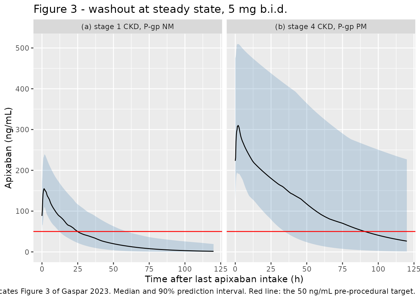
PKNCA validation
NCA is run over the final steady-state dosing interval (228-240 h) for each of the 15 arms.
sim_nca <- sim |>
  dplyr::filter(!is.na(Cc), time <= tau) |>
  dplyr::select(id, time, Cc, arm)

# Guarantee a time = 0 record per (id, arm) so PKNCA can anchor AUC.
sim_nca <- dplyr::bind_rows(
  sim_nca,
  sim_nca |> dplyr::distinct(id, arm) |> dplyr::mutate(time = 0, Cc = 0)
) |>
  dplyr::distinct(id, arm, time, .keep_all = TRUE) |>
  dplyr::arrange(id, arm, time)

conc_obj <- PKNCA::PKNCAconc(sim_nca, Cc ~ time | arm + id)

dose_df <- events |>
  dplyr::filter(evid == 1L) |>
  dplyr::select(id, time, amt, arm)
dose_obj <- PKNCA::PKNCAdose(dose_df, amt ~ time | arm + id)

intervals <- data.frame(
  start = 0, end = 12,
  cmax = TRUE, tmax = TRUE, cmin = TRUE, auclast = TRUE
)

nca_res <- PKNCA::pk.nca(PKNCA::PKNCAdata(conc_obj, dose_obj, intervals = intervals))

nca_summary <- as.data.frame(nca_res) |>
  dplyr::filter(PPTESTCD %in% c("cmax", "tmax", "cmin", "auclast")) |>
  dplyr::group_by(arm, PPTESTCD) |>
  dplyr::summarise(median = median(PPORRES), .groups = "drop") |>
  tidyr::pivot_wider(names_from = PPTESTCD, values_from = median)

knitr::kable(
  nca_summary |>
    dplyr::rename(
      "Arm"                     = arm,
      "Cmax (ng/mL)"            = cmax,
      "Tmax (h)"                = tmax,
      "Cmin (ng/mL)"            = cmin,
      "AUC0-12 (ng*h/mL)"       = auclast
    ),
  digits = 1,
  caption = "Median steady-state NCA parameters over the 12 h dosing interval, apixaban 5 mg b.i.d."
)| Arm | AUC0-12 (ng*h/mL) | Cmax (ng/mL) | Cmin (ng/mL) | Tmax (h) |
|---|---|---|---|---|
| Stage 1 NM | 1434.3 | 162.3 | 88.3 | 1.8 |
| Stage 1 PM | 1457.0 | 157.4 | 92.2 | 1.8 |
| Stage 1 UM | 1061.8 | 139.1 | 61.1 | 1.8 |
| Stage 2 NM | 1672.4 | 180.6 | 107.9 | 1.8 |
| Stage 2 PM | 1907.5 | 204.3 | 129.8 | 1.8 |
| Stage 2 UM | 1334.4 | 156.9 | 78.2 | 1.8 |
| Stage 3 NM | 2138.7 | 212.0 | 132.9 | 1.8 |
| Stage 3 PM | 2492.7 | 238.4 | 167.0 | 2.0 |
| Stage 3 UM | 1831.8 | 201.2 | 113.2 | 2.0 |
| Stage 4 NM | 2672.0 | 264.1 | 187.7 | 1.8 |
| Stage 4 PM | 3168.1 | 314.9 | 221.7 | 1.8 |
| Stage 4 UM | 2597.7 | 256.0 | 179.8 | 1.8 |
| Stage 5 NM | 4012.8 | 367.0 | 300.7 | 2.0 |
| Stage 5 PM | 4419.5 | 413.4 | 333.1 | 1.8 |
| Stage 5 UM | 3518.2 | 324.7 | 255.4 | 2.2 |
Comparison against published NCA
Gaspar 2023 publishes no NCA table of its own. The two NCA-comparable numbers it does report are the terminal half-life of the reference patient and the manufacturer’s Cmin percentile band, so the comparison below uses a typical-value (variability-suppressed) solve, where the half-life is a deterministic property of the model rather than a tmax-selected, NA-prone statistic over a cohort with 88% CV on the peripheral volume.
typ_subj <- tibble::tibble(id = 1L, CRCL = 100, AUC_FEXO = 100.1, OCC = 1L)
typ_events <- dplyr::bind_rows(
  typ_subj |> dplyr::mutate(time = 0, amt = 5, evid = 1L, cmt = "depot",
                            ss = 1L, ii = tau),
  typ_subj |> tidyr::crossing(time = seq(0, 240, by = 0.5)) |>
    dplyr::mutate(amt = NA_real_, evid = 0L, cmt = "central", ss = 0L, ii = 0)
) |>
  dplyr::arrange(time, dplyr::desc(evid))

sim_typ <- rxode2::rxSolve(mod |> rxode2::zeroRe(), events = typ_events,
                           # steady-state searches for long-half-life subjects exceed the default step budget
                           maxsteps = 1e6) |>
  as.data.frame() |>
  dplyr::filter(!is.na(Cc))
#> ℹ parameter labels from comments will be replaced by 'label()'
#> Warning: some etas defaulted to non-mu referenced, possible parsing error: etaiov_cl_1, etaiov_cl_2
#> as a work-around try putting the mu-referenced expression on a simple line
#> Warning: some etas defaulted to non-mu referenced, possible parsing error: etaiov_cl_1, etaiov_cl_2
#> as a work-around try putting the mu-referenced expression on a simple line
#> ℹ omega/sigma items treated as zero: 'etaltlag', 'etalka', 'etalq', 'etalvp', 'etaiov_cl_1', 'etaiov_cl_2'

# Terminal slope fitted well after the washout transient: a time-to-50%
# measured from the moment of withdrawal includes the distribution phase and
# reads long.
# Below 1e-6 of the peak the integrator has no relative accuracy left.
term <- sim_typ |> dplyr::filter(time >= 48, time <= 240, Cc >= 1e-6 * max(Cc))
hl_fit <- log(2) / -coef(lm(log(Cc) ~ time, data = term))[["time"]]

published_nca <- tibble::tibble(
  arm = "Typical patient (CLcr 100 mL/min, P-gp NM)",
  half.life = 17
)
sim_nca_typ <- tibble::tibble(
  arm = "Typical patient (CLcr 100 mL/min, P-gp NM)",
  half.life = hl_fit
)

knitr::kable(
  sim_nca_typ |>
    dplyr::left_join(published_nca, by = "arm", suffix = c("_sim", "_pub")) |>
    dplyr::mutate(`Difference (%)` = 100 * (half.life_sim - half.life_pub) / half.life_pub) |>
    dplyr::rename(
      "NCA parameter"                     = arm,
      "t1/2 simulated (h)"                = half.life_sim,
      "t1/2 published (h)"                = half.life_pub
    ),
  digits = 2,
  caption = "Terminal half-life of the typical patient against the value reported in Gaspar 2023 Results."
)| NCA parameter | t1/2 simulated (h) | t1/2 published (h) | Difference (%) |
|---|---|---|---|
| Typical patient (CLcr 100 mL/min, P-gp NM) | 16.47 | 17 | -3.11 |
Assumptions and deviations
-
The paper’s “45% lower CL” in stage 4 CKD is not reproduced
by its own printed equation, and the equation was followed.
Results, “Covariate analyses” states that a typical P-gp NM patient with
stage 4 CKD (mean CLcr = 22 mL/min) has “45% lower CL” than the same
patient with stage 1 CKD (mean CLcr = 100 mL/min). The Table 2 note
equation with the Table 2 estimate
beta_CLcr = 0.47gives(22/100)^0.47 = 0.491, i.e. 50.9% lower, and no reading of the simulation design recovers 45% either (integrating the power term over uniform CLcr on the stage-4 and stage-1 bands gives 53.8% lower). Recovering exactly 45% would requirebeta_CLcr = 0.395. The abstract’s companion phrasing – “a patient with stage 4 chronic kidney disease would have a 45% higher drug exposure” – is inconsistent with both the equation and with Figure 2, which shows stage 3 already 65-80% higher and stage 5 200-250% higher, bracketing stage 4 far above 45%. The printed equation and the Table 2 point estimates are therefore taken as authoritative and the prose percentage is recorded here as an erratum. The same “45% lower CL” claim appears in the abstract and in Results; both are affected. Every other derived quantity the paper prints – the alpha and beta half-lives, the 78 L total volume, and both P-gp effect sizes – reproduces exactly, which is what makes this one stand out as a slip rather than a transcription error on this side. - Terminal half-lives of 33 h (stage 3) and 52 h (stage 4). Results also reports these as terminal half-lives “on average”. The analytic typical-value terminal half-lives at the stage midpoints (CLcr 44.5 and 22 mL/min, P-gp NM) are 23.4 h and 32.0 h. The gap is consistent with these being means over the simulated cohort, which are inflated by the right skew that log-normal IIV on Q and Vp induces on a half-life; the paper does not state how they were computed, so they are not gated here.
-
The stage-5 Cmin rise depends entirely on an unstated
simulation bound, and is not a model discrepancy. Results
reports that the Cmin increase over normal renal function “reaches up to
200%-250% in patients suffering from stage 5 CKD”. Stage 5 is defined
only as
CLcr < 15 mL/min, with no lower bound stated anywhere in the paper, and the whole claim turns on that missing number: holding everything else fixed, the typical-value rise over stage 1 is 227% at CLcr = 14, 247% at 12.5, 290% at 10, 353% at 7.5 and 457% at 5 mL/min. The paper’s 200-250% therefore corresponds to sampling stage 5 close to its upper edge (CLcr roughly 12.5-14). The cohort here uses 5-15 mL/min and lands at ~290%. Because the target is an artefact of an undocumented choice rather than of the model, it is reported but not gated. -
The P-gp poor-versus-ultra-rapid Cmin difference is larger
than the paper states. Results reports “A 20%-35% difference in
Cmin is expected between P-gp PM and UM patients at all dosage regimens
and CKD stages combined”; the packaged model gives 38-47% across the
five CKD stages, deterministically. The discrepancy is structural rather
than a transcription problem: the clearance ratio between the two
phenotypes is exactly
(285.5/50.4)^-0.17 = 0.745, i.e. a 34.3% clearance difference, which sits squarely inside the paper’s quoted 20-35% band, but a steady-state trough on a 12 h interval responds by more than the clearance ratio, because reduced clearance also lengthens the terminal half-life and so raises the trough. The most likely reading is that the quoted range describes the clearance effect rather than the simulated Cmin effect. Both P-gp effect sizes on clearance itself (-16% for PM, +12% for UM versus NM) reproduce exactly, as the deterministic-checks section shows, so the covariate transcription is confirmed independently of this claim. Reported but not gated. - P-glycoprotein covariate distribution. Methods, “Model-based simulations” states only that “a uniform distribution in the studied range was assumed for all covariates”, without giving a range for the fexofenadine AUC(2-6 h) index within each phenotype category. Methods, “Phenotyping” gives category mean +/- SD, so the cohort here draws uniformly over mean +/- SD (PM 218.4-352.6, NM 52.6-147.6, UM 35.1-65.7 mg*h/L). This choice affects the width of the simulated distributions but not their centres, which are what the gates above test.
- CKD band endpoints. Stage 1 is defined by an open-ended CLcr > 90 mL/min and is capped here at the observed cohort maximum of 136 mL/min (Table 1); stage 5 is defined by CLcr < 15 mL/min and is bounded below at 5 mL/min. Both stage 4 (15-29) and stage 5 extend below the observed cohort minimum of 23 mL/min, so those two strata are extrapolation beyond the fitted range – as they are in the paper’s own simulations.
-
Occasion. Each simulated patient is given
OCC = 1, i.e. a single hospitalization, which is the modal case in the source data (94 of 100 patients). Because the paper estimates one shared inter-occasion variance, the second occasion’s variance isfix()ed equal to the first in the model file and a two-occasion patient would simply draw a second, independent clearance offset. -
Bioavailability. All disposition parameters are
apparent (CL/F, Vc/F, Q/F, Vp/F), as the paper labels them; F is not
identifiable from oral-only data. No
f(depot)term is applied, so absolute volumes and clearances are not directly comparable with intravenous apixaban literature values. -
Dried blood spots. The fitted concentrations are
plasma values back- calculated from dried blood spots via
Conc_plasma = Conc_DBS * 1.46 + 13.84(Foerster et al., cited by Gaspar 2023 Methods). That affine transformation is a property of the assay, not of the model, and is not re-applied here. -
Covariates screened but not retained. Body weight,
age, sex, smoking status, urea, albumin, AST, ALT, alkaline phosphatase,
gamma-glutamyl transferase, bilirubin and CYP3A4/5 phenotypic activity
were all tested and none was retained; the paper publishes no point
estimate for any of them. They are recorded in the model file’s
covariatesDataExcludedmetadata rather than incovariateData. Note in particular that body weight and age reach clearance throughCRCL, since both are inputs to the Cockcroft-Gault equation – the Discussion makes this argument explicitly – so a user must not add a separate allometric weight term on top of this model. -
No non-paper-derived parameter values. Every value
in
ini()comes from Gaspar 2023 Table 2 or from the constants printed in the Table 2 note and Methods. Nothing was digitised from a figure, obtained by correspondence, or carried from an upstream model.