Cefazolin (Gebreyesus 2024)
Source:vignettes/articles/Gebreyesus_2024_cefazolin.Rmd
Gebreyesus_2024_cefazolin.RmdModel and source
- Citation: Gebreyesus MS, Dresner A, Wiesner L, Coetzee E, Verschuuren T, Wasmann R, Denti P. Dose optimization of cefazolin in South African children undergoing cardiac surgery with cardiopulmonary bypass. CPT Pharmacometrics Syst Pharmacol 2024;13(9):1595-1605. doi:10.1002/psp4.13196.
- Description: Two-compartment IV population PK model for total plasma cefazolin in South African children under 25 kg undergoing cardiac surgery with cardiopulmonary bypass (CPB), with a third compartment for the CPB circuit. The circuit compartment exchanges with the central compartment only while the patient is on bypass; its volume is the circuit priming volume and its flow a fixed adult cardiac output (336 L/h, allometric to 70 kg), both multiplied by an estimated scaling factor (0.679). Clearances and volumes scale allometrically on body weight (reference 10 kg) and clearance is proportional to bedside-Schwartz eGFR (reference 120 mL/min/1.73 m^2). A dose added to the CPB priming fluid is a bolus into the circuit compartment.
- Article: https://doi.org/10.1002/psp4.13196 (open access; PMC11881764)
Gebreyesus and colleagues modelled total plasma cefazolin in 22 children under 25 kg undergoing cardiac surgery with cardiopulmonary bypass (CPB) in Cape Town, then used the model to compare the hospital’s 50 mg/kg every-4-hour bolus regimen against a continuous infusion whose loading and maintenance doses are computed from the model’s typical clearance and steady-state volume. The NONMEM control stream is published as Supplementary Material S3, and every value below is taken from it and from Table 3, which agree.
The CPB circuit is a third compartment. While the patient is connected, drug exchanges between the central compartment and the circuit at a flow fixed to an adult cardiac output (336 L/h, scaled allometrically from 70 kg), and the circuit volume is the priming volume; an estimated factor (0.679) multiplies both, which the authors note is close to the plasma fraction of whole blood. A dose added to the priming fluid is a bolus into the circuit compartment. When the patient comes off bypass the exchange stops and whatever drug is in the circuit stays there.
Population
Twenty-two children (13 male, 9 female) aged 1-94 months (median 17), weighing 2.0-22 kg (median 8.5) and with bedside-Schwartz eGFR 48-159 mL/min/1.73 m^2 (median 116) contributed 249 plasma concentrations (Table 2). They underwent surgery for congenital heart disease such as atrioventricular septal defect, pulmonary atresia and tetralogy of Fallot; surgical duration was 2.38 (0.567-5.63) h and priming volume 0.40 (0.25-0.55) L. Each child received 50 mg/kg cefazolin by 45-second IV injection after induction and again 4-6 h later (at most three doses); six also had 50 mg/kg added to the CPB priming fluid.
The same information is available programmatically via
readModelDb("Gebreyesus_2024_cefazolin")()$population.
Source trace
| Equation / parameter | Value | Source location |
|---|---|---|
lcl |
log(0.856) L/h | Table 3 ‘Clearance’; S3 THETA(1)
|
lvc |
log(1.07) L | Table 3 ‘Central volume of distribution’; S3
THETA(2)
|
lq |
log(1.41) L/h | Table 3 ‘Intercompartmental clearance’; S3
THETA(6)
|
lvp |
log(1.61) L | Table 3 ‘Peripheral volume of distribution’; S3
THETA(5)
|
qbfr |
336 L/h, fixed | Table 3 ‘Intercompartmental clearance for CPB compartment’; S3
THETA(7)
|
fcircuit |
0.679 | Table 3 ‘Scaling factor for the CPB compartment’; S3
THETA(8)
|
e_wt_cl_q |
0.75, fixed | S1 ‘Population pharmacokinetic modelling’; S3
ALLMCL_WT, ALLMQ2
|
e_wt_vc_vp |
1, fixed | S1; S3 ALLMV_WT
|
etalcl |
0.0523 | S3 $OMEGA (Table 3: 23.2% CV) |
etalvc |
0.033 | S3 $OMEGA (Table 3: 18.3% CV) |
etalvp |
0.0779 | S3 $OMEGA (Table 3: 28.5% CV) |
propSd |
0.155 | Table 3 ‘Proportional error’; S3 THETA(3)
|
addSd |
0.1172 mg/L, fixed | Table 3 footnote f (20% of LLOQ 0.586 mg/L); S3
ADD = THETA(4) + LLOQ*0.2
|
cl = TVCL (WT/10)^0.75 (CRCL/120) |
n/a | Results equation; S3 TVCL
|
vc, vp = TV (WT/10)
|
n/a | Results equation; S3 TVV, TVV2
|
q = TVQ (WT/10)^0.75 (no BSV) |
n/a | S3 TVQ, Q = TVQ
|
circuit flow 336 (WT/70)^0.75 x 0.679
|
n/a | Results; S3 Q2 = TVQ2*THETA(8)
|
circuit volume CIRCUIT_PRIME_VOL x 0.679
|
n/a | S3 V3 = VCPB0*THETA(8)
|
d/dt(...) with the circuit terms gated by the CPB
switch |
n/a | S3 $DES
|
eGFR 0.413 x HT / SCr
|
n/a | S1 Eq. 1; S3 CRCL_SCHW
|
Cc ~ add + prop, combined2 |
n/a | S3 W = SQRT(ADD**2+PROP**2)
|
Dose calculator (Tables 1, S1 and S2)
The continuous-infusion regimen sets the loading dose to
Vss x 100 mg/L and the hourly maintenance rate to
CL x 100 mg/L, using the population-predicted parameters
for the child’s weight and eGFR (Table 1). Supplementary Table S1 works
the example for a 2 kg child with eGFR 50. The model’s typical values
reproduce it exactly.
mod <- readModelDb("Gebreyesus_2024_cefazolin")
mod_typical <- rxode2::zeroRe(mod)
#> ℹ parameter labels from comments will be replaced by 'label()'

typical_params <- function(WT, CRCL) {
  ev <- data.frame(
    id = seq_along(WT), time = 0, evid = 0L, amt = 0, cmt = "central",
    WT = WT, CRCL = CRCL, CPB_ON = 0L, CPB_REWARM = 0L, CIRCUIT_PRIME_VOL = 0.4
  )
  sim <- as.data.frame(rxode2::rxSolve(mod_typical, ev, returnType = "data.frame"))
  # rxSolve drops the id column when there is a single subject
  if (!"id" %in% names(sim)) sim$id <- 1L
  dplyr::transmute(sim, id, cl, vss = vc + vp)
}

c_target <- 100 # mg/L (Methods)
s1 <- typical_params(WT = 2, CRCL = 50) |>
  dplyr::mutate(
    loading_mg = vss * c_target,
    maint_mg_h = cl * c_target,
    cpb_dose_mg = 0.5 * loading_mg
  )
#> ℹ omega/sigma items treated as zero: 'etalcl', 'etalvc', 'etalvp'
s1_published <- c(vss = 0.536, cl = 0.107, loading_mg = 53.6, maint_mg_h = 10.7, cpb_dose_mg = 26.8)
s1_model <- unlist(s1[names(s1_published)])
knitr::kable(
  data.frame(
    Quantity = c("Vss (L)", "CL (L/h)", "Loading dose (mg)", "Maintenance (mg/h)", "CPB dose (mg)"),
    Model = signif(s1_model, 3),
    `Table S1` = s1_published,
    check.names = FALSE
  ),
  caption = "Replicates Supplementary Table S1 (2 kg, eGFR 50 mL/min/1.73 m^2)."
)| Quantity | Model | Table S1 | |
|---|---|---|---|
| vss | Vss (L) | 0.536 | 0.536 |
| cl | CL (L/h) | 0.107 | 0.107 |
| loading_mg | Loading dose (mg) | 53.600 | 53.600 |
| maint_mg_h | Maintenance (mg/h) | 10.700 | 10.700 |
| cpb_dose_mg | CPB dose (mg) | 26.800 | 26.800 |
# Same equations evaluated on both sides; only the table's 3-digit rounding differs.
stopifnot(all(abs(s1_model / s1_published - 1) < 0.005))
Supplementary Table S2 lists, for each of the 22 study patients, the total cefazolin given over 12 h by each regimen. The continuous-infusion totals are the loading dose plus the maintenance rate over the 11 h 40 min between the start of the infusion (20 min after induction) and the end of the 12-h window.
table_s2 <- tibble::tribble(
  ~patient, ~WT, ~CRCL, ~standard_mg, ~alternative_mg,
  1, 2, 48, 300, 174,
  2, 5.5, 81, 825, 580,
  3, 5.9, 85, 885, 635,
  4, 5.4, 91, 810, 623,
  5, 8.4, 97, 1260, 933,
  6, 6, 97, 900, 713,
  7, 5.3, 99, 795, 655,
  8, 8.9, 108, 1335, 1063,
  9, 11.8, 108, 1770, 1337,
  10, 10, 114, 1500, 1213,
  11, 8.5, 116, 1275, 1080,
  12, 9.4, 117, 1410, 1177,
  13, 18.7, 119, 2805, 2080,
  14, 10, 128, 1500, 1331,
  15, 7.8, 129, 1170, 1103,
  16, 12.5, 131, 1875, 1620,
  17, 6.3, 131, 945, 938,
  18, 8.1, 132, 1215, 1156,
  19, 17, 135, 2550, 2125,
  20, 21.6, 140, 3240, 2651,
  21, 14, 145, 2100, 1924,
  22, 12.6, 159, 1890, 1915
)
infusion_h <- 12 - 20 / 60
s2_check <- typical_params(table_s2$WT, table_s2$CRCL) |>
  dplyr::mutate(
    model_alternative_mg = vss * c_target + cl * c_target * infusion_h,
    model_standard_mg = 3 * 50 * table_s2$WT
  ) |>
  dplyr::bind_cols(table_s2 |> dplyr::select(-patient)) |>
  dplyr::mutate(pct_diff = 100 * (model_alternative_mg / alternative_mg - 1))
#> ℹ omega/sigma items treated as zero: 'etalcl', 'etalvc', 'etalvp'
#> Warning: multi-subject simulation without without 'omega'
s2_check |>
  dplyr::transmute(
    Patient = id, `Weight (kg)` = WT, `eGFR` = CRCL,
    `Standard, Table S2 (mg)` = standard_mg, `Standard, model (mg)` = model_standard_mg,
    `Infusion, Table S2 (mg)` = alternative_mg,
    `Infusion, model (mg)` = round(model_alternative_mg),
    `Difference (%)` = round(pct_diff, 2)
  ) |>
knitr::kable(caption = "Replicates Supplementary Table S2 (totals over 12 h, no CPB dose).")| Patient | Weight (kg) | eGFR | Standard, Table S2 (mg) | Standard, model (mg) | Infusion, Table S2 (mg) | Infusion, model (mg) | Difference (%) |
|---|---|---|---|---|---|---|---|
| 1 | 2.0 | 48 | 300 | 300 | 174 | 173 | -0.54 |
| 2 | 5.5 | 81 | 825 | 825 | 580 | 578 | -0.36 |
| 3 | 5.9 | 85 | 885 | 885 | 635 | 634 | -0.11 |
| 4 | 5.4 | 91 | 810 | 810 | 623 | 622 | -0.20 |
| 5 | 8.4 | 97 | 1260 | 1260 | 933 | 933 | 0.05 |
| 6 | 6.0 | 97 | 900 | 900 | 713 | 711 | -0.26 |
| 7 | 5.3 | 99 | 795 | 795 | 655 | 654 | -0.18 |
| 8 | 8.9 | 108 | 1335 | 1335 | 1063 | 1062 | -0.08 |
| 9 | 11.8 | 108 | 1770 | 1770 | 1337 | 1334 | -0.24 |
| 10 | 10.0 | 114 | 1500 | 1500 | 1213 | 1217 | 0.31 |
| 11 | 8.5 | 116 | 1275 | 1275 | 1080 | 1082 | 0.22 |
| 12 | 9.4 | 117 | 1410 | 1410 | 1177 | 1181 | 0.38 |
| 13 | 18.7 | 119 | 2805 | 2805 | 2080 | 2085 | 0.23 |
| 14 | 10.0 | 128 | 1500 | 1500 | 1331 | 1333 | 0.17 |
| 15 | 7.8 | 129 | 1170 | 1170 | 1103 | 1100 | -0.26 |
| 16 | 12.5 | 131 | 1875 | 1875 | 1620 | 1624 | 0.24 |
| 17 | 6.3 | 131 | 945 | 945 | 938 | 940 | 0.19 |
| 18 | 8.1 | 132 | 1215 | 1215 | 1156 | 1155 | -0.08 |
| 19 | 17.0 | 135 | 2550 | 2550 | 2125 | 2128 | 0.15 |
| 20 | 21.6 | 140 | 3240 | 3240 | 2651 | 2655 | 0.14 |
| 21 | 14.0 | 145 | 2100 | 2100 | 1924 | 1928 | 0.22 |
| 22 | 12.6 | 159 | 1890 | 1890 | 1915 | 1911 | -0.19 |
Typical profiles of the smallest patient (Figures S2 and S3)
The authors simulated the smallest study patient (2 kg, eGFR 50) through a 12-h dosing period with the circuit connected from 1 to 6.5 h (the grey band in Figures S2 and S3) and the 0.4 L priming volume the hospital uses below 10 kg. The standard regimen is 100 mg at 0, 4 and 8 h, with an optional 100 mg CPB dose; the continuous infusion is a 53.6 mg loading dose and 10.7 mg/h from 20 min, with an optional 26.8 mg CPB dose (Table S1). The CPB dose is placed in the circuit at the moment of connection.
cpb_start <- 1
cpb_end <- 6.5
cpb_switch <- function(time) as.integer(time >= cpb_start & time < cpb_end)

make_events <- function(doses, WT, CRCL, prime, obs_times, id = 1L) {
  obs <- data.frame(time = obs_times, evid = 0L, amt = 0, rate = 0, cmt = "central")
  dplyr::bind_rows(doses, obs) |>
    dplyr::mutate(
      id = id, WT = WT, CRCL = CRCL, CIRCUIT_PRIME_VOL = prime,
      CPB_ON = cpb_switch(time), CPB_REWARM = 0L
    ) |>
    dplyr::arrange(time, dplyr::desc(evid))
}

regimen_doses <- function(regimen, WT, loading, maint) {
  bolus <- 50 * WT
  std <- data.frame(time = c(0, 4, 8), evid = 1L, amt = bolus, rate = 0, cmt = "central")
  ci <- data.frame(
    time = c(0, 20 / 60), evid = 1L,
    amt = c(loading, maint * infusion_h), rate = c(0, maint), cmt = "central"
  )
  cpb <- function(amt) data.frame(time = cpb_start, evid = 1L, amt = amt, rate = 0, cmt = "circuit_plasma")
  switch(regimen,
    "Standard" = std,
    "Standard + CPB dose" = dplyr::bind_rows(std, cpb(bolus)),
    "Infusion" = ci,
    "Infusion + CPB dose" = dplyr::bind_rows(ci, cpb(0.5 * loading))
  )
}

regimens <- c("Standard", "Standard + CPB dose", "Infusion", "Infusion + CPB dose")
fine_times <- sort(unique(c(seq(0, 12, by = 0.02), 0.999, 3.999, 6.499, 7.999)))
small <- lapply(seq_along(regimens), function(i) {
  ev <- make_events(
    regimen_doses(regimens[i], WT = 2, loading = s1$loading_mg, maint = s1$maint_mg_h),
    WT = 2, CRCL = 50, prime = 0.4, obs_times = fine_times, id = i
  )
  as.data.frame(rxode2::rxSolve(mod_typical, ev, returnType = "data.frame")) |>
    dplyr::mutate(regimen = regimens[i])
}) |>
  dplyr::bind_rows()
#> ℹ omega/sigma items treated as zero: 'etalcl', 'etalvc', 'etalvp'
#> ℹ omega/sigma items treated as zero: 'etalcl', 'etalvc', 'etalvp'
#> ℹ omega/sigma items treated as zero: 'etalcl', 'etalvc', 'etalvp'
#> ℹ omega/sigma items treated as zero: 'etalcl', 'etalvc', 'etalvp'

ggplot(small, aes(time, Cc)) +
  annotate("rect", xmin = cpb_start, xmax = cpb_end, ymin = 0, ymax = Inf, alpha = 0.2) +
  geom_line(colour = "purple") +
  geom_hline(yintercept = c(40, 360), colour = "red") +
  facet_wrap(~regimen) +
  labs(
    x = "Time after first dose (h)", y = "Cefazolin concentration (mg/L)",
    caption = "Replicates Figures S2 and S3 of Gebreyesus 2024 (grey: connected to CPB)."
  )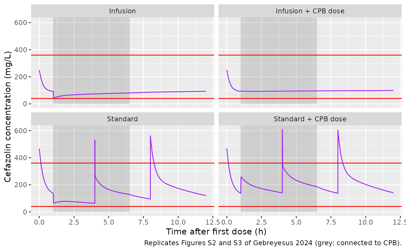
The maintainers read the concentrations at the troughs and band edges off Figures S2 and S3 (peaks are not compared: the published curves are drawn on a grid too coarse to resolve the instant after a bolus).
digitised <- tibble::tribble(
  ~regimen, ~time, ~published,
  "Standard", 0.999, 133,
  "Standard", 3.999, 60,
  "Standard", 6.499, 128,
  "Standard", 7.999, 95,
  "Standard", 12, 118,
  "Standard + CPB dose", 3.999, 140,
  "Standard + CPB dose", 6.499, 185,
  "Standard + CPB dose", 7.999, 138,
  "Standard + CPB dose", 12, 142,
  "Infusion", 0.999, 90,
  "Infusion", 6.499, 80,
  "Infusion", 12, 92,
  "Infusion + CPB dose", 6.499, 95,
  "Infusion + CPB dose", 12, 98
)
small_check <- digitised |>
  dplyr::left_join(small |> dplyr::select(regimen, time, Cc), by = c("regimen", "time")) |>
  dplyr::mutate(pct_diff = 100 * (Cc / published - 1))
knitr::kable(small_check, digits = 1, caption = "Typical-value concentrations (mg/L) vs Figures S2 and S3.")| regimen | time | published | Cc | pct_diff |
|---|---|---|---|---|
| Standard | 1.0 | 133 | 137.4 | 3.3 |
| Standard | 4.0 | 60 | 62.8 | 4.6 |
| Standard | 6.5 | 128 | 128.8 | 0.6 |
| Standard | 8.0 | 95 | 94.7 | -0.3 |
| Standard | 12.0 | 118 | 120.5 | 2.1 |
| Standard + CPB dose | 4.0 | 140 | 140.6 | 0.5 |
| Standard + CPB dose | 6.5 | 185 | 185.5 | 0.2 |
| Standard + CPB dose | 8.0 | 138 | 136.6 | -1.0 |
| Standard + CPB dose | 12.0 | 142 | 140.7 | -0.9 |
| Infusion | 1.0 | 90 | 92.4 | 2.6 |
| Infusion | 6.5 | 80 | 80.6 | 0.7 |
| Infusion | 12.0 | 92 | 93.1 | 1.2 |
| Infusion + CPB dose | 6.5 | 95 | 95.8 | 0.8 |
| Infusion + CPB dose | 12.0 | 98 | 98.5 | 0.5 |
Probability of target attainment (Figure 3)
The efficacy target is a free concentration above 4 x MIC for the whole 12-h period; with a free fraction of 0.2 the total-concentration threshold is 20 x MIC (40 mg/L at the MSSA cutoff of 2 mg/L). Figure 3 shows the standard regimen failing worst in small children with high eGFR. The paper used 1000 virtual patients per weight and renal-function group; this vignette simulates the most discriminating row of the figure (eGFR 130 mL/min/1.73 m^2) with 200 children per weight band and regimen, weight uniform within each band, and the hospital’s priming volumes (0.4 L below 10 kg, 0.6 L for 10-20 kg, 0.8 L above).
rxode2::rxSetSeed(2024)
n_per_arm <- 200
weight_bands <- tibble::tribble(
  ~band, ~lo, ~hi,
  "<5 kg", 2, 5,
  "5-10 kg", 5, 10,
  "10-15 kg", 10, 15,
  "15-20 kg", 15, 20,
  "20-25 kg", 20, 25
)
# Troughs fall just before the 4 h and 8 h doses, at 12 h, and in the dip
# just after connection to the circuit at 1 h.
pta_times <- sort(unique(c(seq(0, 12, by = 0.05), seq(1, 1.3, by = 0.01), 3.999, 7.999)))
theta <- rxode2::rxode2(mod)$theta
#> ℹ parameter labels from comments will be replaced by 'label()'
arm_grid <- tidyr::expand_grid(band = weight_bands$band, regimen = regimens)

pta_events <- lapply(seq_len(nrow(arm_grid)), function(a) {
  wb <- weight_bands[weight_bands$band == arm_grid$band[a], ]
  wts <- stats::runif(n_per_arm, wb$lo, wb$hi)
  lapply(seq_len(n_per_arm), function(j) {
    WT <- wts[j]
    loading <- (exp(theta[["lvc"]]) + exp(theta[["lvp"]])) * (WT / 10) * c_target
    maint <- exp(theta[["lcl"]]) * (WT / 10)^0.75 * (130 / 120) * c_target
    prime <- if (WT < 10) 0.4 else if (WT < 20) 0.6 else 0.8
    make_events(
      regimen_doses(arm_grid$regimen[a], WT, loading, maint),
      WT = WT, CRCL = 130, prime = prime, obs_times = pta_times,
      id = (a - 1L) * n_per_arm + j
    ) |>
      dplyr::mutate(band = arm_grid$band[a], regimen = arm_grid$regimen[a])
  }) |>
    dplyr::bind_rows()
}) |>
  dplyr::bind_rows()
stopifnot(!anyDuplicated(unique(pta_events[, c("id", "time", "evid", "cmt")])))

pta_sim <- rxode2::rxSolve(mod, pta_events, keep = c("band", "regimen"), returnType = "data.frame") |>
  as.data.frame()
#> ℹ parameter labels from comments will be replaced by 'label()'
Cc is the individual prediction without residual error,
which is what a target-attainment simulation evaluates.
mic <- c(0.125, 0.25, 0.5, 1, 2)
# The t = 0 row follows the first bolus, so it is a peak, not a trough.
cmin_by_id <- pta_sim |>
  dplyr::group_by(id, band, regimen) |>
  dplyr::summarise(cmin = min(Cc), .groups = "drop")
pta <- tidyr::expand_grid(cmin_by_id, mic = mic) |>
  dplyr::group_by(band, regimen, mic) |>
  dplyr::summarise(pta = 100 * mean(cmin > 20 * mic), .groups = "drop") |>
  dplyr::mutate(band = factor(band, levels = weight_bands$band))

ggplot(pta, aes(factor(mic), pta, colour = regimen, group = regimen)) +
  geom_line() +
  geom_point() +
  geom_hline(yintercept = 90, linetype = "dashed") +
  facet_wrap(~band, nrow = 1) +
  labs(
    x = "MIC for MSSA (mg/L)", y = "PTA (%)", colour = NULL,
    caption = "Replicates the eGFR 130 mL/min/1.73 m^2 row of Figure 3 of Gebreyesus 2024."
  ) +
  theme(legend.position = "bottom")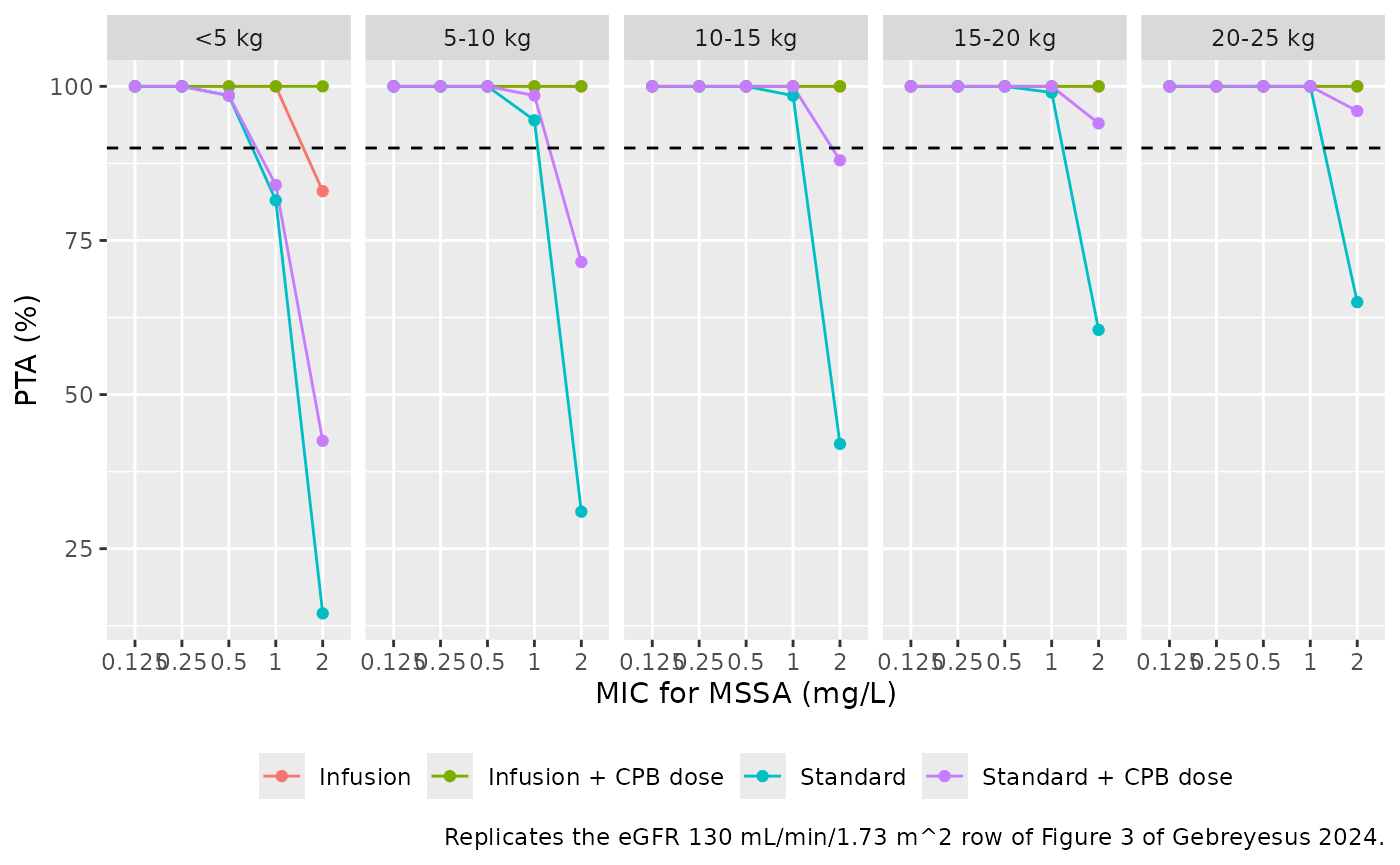
The maintainers read the MIC 2 mg/L points of that row off Figure 3.
pta_published <- tibble::tribble(
  ~band, ~regimen, ~published,
  "<5 kg", "Standard", 15,
  "5-10 kg", "Standard", 35,
  "10-15 kg", "Standard", 50,
  "15-20 kg", "Standard", 62,
  "20-25 kg", "Standard", 67,
  "<5 kg", "Standard + CPB dose", 52,
  "5-10 kg", "Standard + CPB dose", 75,
  "10-15 kg", "Standard + CPB dose", 86,
  "15-20 kg", "Standard + CPB dose", 91,
  "20-25 kg", "Standard + CPB dose", 94
)
pta_check <- pta |>
  dplyr::filter(mic == 2) |>
  dplyr::mutate(band = as.character(band)) |>
  dplyr::left_join(pta_published, by = c("band", "regimen")) |>
  dplyr::mutate(diff_pp = pta - published) |>
  dplyr::arrange(regimen, factor(band, levels = weight_bands$band))
pta_check |>
  dplyr::rename(`Weight band` = band, Regimen = regimen, `MIC (mg/L)` = mic,
                `PTA, simulated (%)` = pta, `PTA, Figure 3 (%)` = published,
                `Difference (pp)` = diff_pp) |>
knitr::kable(digits = 1, caption = "PTA at MIC 2 mg/L, eGFR 130 mL/min/1.73 m^2.")| Weight band | Regimen | MIC (mg/L) | PTA, simulated (%) | PTA, Figure 3 (%) | Difference (pp) |
|---|---|---|---|---|---|
| <5 kg | Infusion | 2 | 83.0 | NA | NA |
| 5-10 kg | Infusion | 2 | 100.0 | NA | NA |
| 10-15 kg | Infusion | 2 | 100.0 | NA | NA |
| 15-20 kg | Infusion | 2 | 100.0 | NA | NA |
| 20-25 kg | Infusion | 2 | 100.0 | NA | NA |
| <5 kg | Infusion + CPB dose | 2 | 100.0 | NA | NA |
| 5-10 kg | Infusion + CPB dose | 2 | 100.0 | NA | NA |
| 10-15 kg | Infusion + CPB dose | 2 | 100.0 | NA | NA |
| 15-20 kg | Infusion + CPB dose | 2 | 100.0 | NA | NA |
| 20-25 kg | Infusion + CPB dose | 2 | 100.0 | NA | NA |
| <5 kg | Standard | 2 | 14.5 | 15 | -0.5 |
| 5-10 kg | Standard | 2 | 31.0 | 35 | -4.0 |
| 10-15 kg | Standard | 2 | 42.0 | 50 | -8.0 |
| 15-20 kg | Standard | 2 | 60.5 | 62 | -1.5 |
| 20-25 kg | Standard | 2 | 65.0 | 67 | -2.0 |
| <5 kg | Standard + CPB dose | 2 | 42.5 | 52 | -9.5 |
| 5-10 kg | Standard + CPB dose | 2 | 71.5 | 75 | -3.5 |
| 10-15 kg | Standard + CPB dose | 2 | 88.0 | 86 | 2.0 |
| 15-20 kg | Standard + CPB dose | 2 | 94.0 | 91 | 3.0 |
| 20-25 kg | Standard + CPB dose | 2 | 96.0 | 94 | 2.0 |
bolus_rows <- pta_check |> dplyr::filter(!is.na(published))
infusion_rows <- pta_check |> dplyr::filter(grepl("Infusion", regimen))
stopifnot(
  # Centre: a mis-scaled clearance or circuit volume shifts every band by tens
  # of points; 200 per arm gives a Monte Carlo SE of at most 3.5 points.
  abs(median(bolus_rows$diff_pp)) < 10,
  # Envelope across the ten bolus arms, robust to which arm sits in a tail.
  quantile(abs(bolus_rows$diff_pp), 0.9) < 20,
  # Figure 3: the infusion regimens attain the target in essentially every child.
  median(infusion_rows$pta) > 95
)
One arm departs from the figure: the infusion without a CPB dose in children under 5 kg reaches about 85% here against about 97% in Figure 3. In these children the circuit volume (0.4 L x 0.679) is comparable to the central volume, so concentrations fall by roughly half the moment the circuit is connected and recover within minutes (the dip in Figure S3). The simulation above looks for the minimum on a 0.01-h grid around connection; on a coarser grid the dip is missed and the PTA rises to the published value, which suggests the paper evaluated attainment on a coarser grid. The paper does not state its grid, so the comparison is shown rather than asserted.
grid_pta <- lapply(c(0.01, 0.05, 0.1, 0.25), function(step) {
  pta_sim |>
    dplyr::filter(band == "<5 kg", regimen == "Infusion", abs(time / step - round(time / step)) < 1e-6) |>
    dplyr::group_by(id) |>
    dplyr::summarise(cmin = min(Cc), .groups = "drop") |>
    dplyr::summarise(`Grid step (h)` = step, `PTA at MIC 2 (%)` = 100 * mean(cmin > 40))
}) |>
  dplyr::bind_rows()
knitr::kable(grid_pta, digits = c(2, 1), caption = "Infusion without CPB dose, < 5 kg, eGFR 130: PTA by evaluation grid.")| Grid step (h) | PTA at MIC 2 (%) |
|---|---|
| 0.01 | 83.0 |
| 0.05 | 86.0 |
| 0.10 | 90.5 |
| 0.25 | 98.0 |
PKNCA
The paper reports no NCA parameters; Figure S6 shows trough and average concentrations only as box plots. The block below computes the 12-h exposure of the 10-15 kg band at eGFR 130 per regimen, on a 0.25-h subsample of the simulation grid, so the regimens can be compared on peak, average and AUC. The time-zero row is the simulated concentration just after the first bolus.
nca_conc <- pta_sim |>
  dplyr::filter(band == "10-15 kg", !is.na(Cc), abs(time / 0.25 - round(time / 0.25)) < 1e-6) |>
  dplyr::select(id, time, Cc, regimen)
nca_conc <- dplyr::bind_rows(
  nca_conc,
  nca_conc |> dplyr::distinct(id, regimen) |> dplyr::mutate(time = 0, Cc = 0)
) |>
  dplyr::distinct(id, regimen, time, .keep_all = TRUE) |>
  dplyr::arrange(id, regimen, time)

nca_dose <- pta_events |>
  dplyr::filter(band == "10-15 kg", evid == 1, cmt == "central") |>
  dplyr::group_by(id, regimen) |>
  dplyr::slice(1) |>
  dplyr::ungroup() |>
  dplyr::select(id, time, amt, regimen)

conc_obj <- PKNCA::PKNCAconc(nca_conc, Cc ~ time | regimen + id)
dose_obj <- PKNCA::PKNCAdose(nca_dose, amt ~ time | regimen + id)
intervals <- data.frame(start = 0, end = 12, auclast = TRUE, cav = TRUE, cmax = TRUE)
nca_res <- PKNCA::pk.nca(PKNCA::PKNCAdata(conc_obj, dose_obj, intervals = intervals))

nca_summary <- as.data.frame(nca_res$result) |>
  dplyr::filter(PPTESTCD %in% c("auclast", "cav", "cmax")) |>
  dplyr::group_by(regimen, PPTESTCD) |>
  dplyr::summarise(median = stats::median(PPORRES), .groups = "drop") |>
  tidyr::pivot_wider(names_from = PPTESTCD, values_from = median)
nca_summary |>
  dplyr::select(regimen, cmax, cav, auclast) |>
  dplyr::rename(
    Regimen = regimen, `Cmax (mg/L)` = cmax,
    `Cav 0-12 (mg/L)` = cav, `AUC0-12 (mg*h/L)` = auclast
  ) |>
knitr::kable(digits = 1, caption = "Median simulated 12-h exposure, 10-15 kg, eGFR 130.")| Regimen | Cmax (mg/L) | Cav 0-12 (mg/L) | AUC0-12 (mg*h/L) |
|---|---|---|---|
| Infusion | 250.6 | 97.2 | 1166.0 |
| Infusion + CPB dose | 246.5 | 105.9 | 1270.7 |
| Standard | 521.9 | 127.9 | 1534.4 |
| Standard + CPB dose | 579.1 | 177.7 | 2132.0 |
# Cav of the infusion arm is set by design near the 100 mg/L target.
cav_infusion <- nca_summary$cav[nca_summary$regimen == "Infusion"]
stopifnot(cav_infusion > 70, cav_infusion < 130)
Assumptions and deviations
-
CPB switch. The control stream turns the circuit on
at the start of bypass and off at its end with a single data item and
does not split out rewarming. The model uses
CPB_ON + CPB_REWARMas the switch, so the circuit is connected whenever the patient is on bypass in either phase; a user with no separate rewarming record setsCPB_ON = 1for the whole bypass run. -
eGFR as an input. The control stream computes eGFR
from height and serum creatinine (bedside Schwartz, 0.413 x HT / SCr).
The model takes that value as the
CRCLcolumn, which is how the paper’s own dose calculator and simulations specify renal function. -
CPB dose timing. The control stream loads the CPB
dose into the circuit compartment as its initial amount; the vignette
gives it as a bolus into
circuit_plasmaat the moment of connection, which is equivalent because the circuit is isolated until then. - Figure S3 caption. The caption gives the infusion regimen’s CPB dose as 50 mg/kg, while the Methods and Table S1 give 0.5 x loading dose (26.8 mg for the 2 kg child); the vignette uses 26.8 mg, and the resulting curve matches the figure.
- Virtual population. The paper’s 5000-child virtual population (from its reference 24) is not available. Weight is drawn uniformly within each band, with the smallest band starting at 2 kg (the smallest study patient), and only the eGFR 130 row of Figure 3 is simulated, at 200 children per arm.
- Attainment grid. Attainment is judged on the minimum concentration over a 0.05-h grid refined to 0.01 h around connection to the circuit; the paper does not state its grid (see the infusion arm under 5 kg above).
- Digitised values. The comparison values for Figures S2, S3 and 3 were read off the published figures by the maintainers.
- Errata. No correction notice for this article was found in Europe PMC as of 2026-11-03.