Model and source
- Citation: Yin A, Ettaieb MHT, Swen JJ, van Deun L, Kerkhofs TMA, van der Straaten RJHM, Corssmit EPM, Gelderblom H, Kerstens MN, Feelders RA, Eekhoff M, Timmers HJLM, D’Avolio A, Cusato J, Guchelaar HJ, Haak HR, Moes DJAR. Population pharmacokinetic and pharmacogenetic analysis of mitotane in patients with adrenocortical carcinoma: towards individualized dosing. Clin Pharmacokinet. 2021;60(1):89-102. doi:10.1007/s40262-020-00913-y. Parameter estimates from Table 2 (final model) and its footnotes a-c; IIV / IOV / residual-error equations (Eqs. S1-S2) and covariate forms (Eqs. S4-S5) from Online Resource 1. The Boer lean-body-weight coefficients, the standard-deviation scale of the printed CV% values and the ODE system are taken from the authors’ published Shiny app script (github.com/AnyueYin/Shiny-app-script-for-model-simulation—Population-PK-and-PG-analysis-of-mitotane).
- Description: Two-compartment population PK model with first-order absorption for oral mitotane in adults with adrenocortical carcinoma (Yin 2021), final pharmacogenetic model. Apparent clearance carries a power effect of lean body weight (Boer formula, derived from weight, height and sex) plus multiplicative genotype effects of CYP2C19*2 (rs4244285) carriage, SLCO1B3 699A>G (rs7311358) G-allele carriage and SLCO1B1 571T>C (rs4149057) CC or TT genotype (TC reference); apparent central volume carries a power effect of fat amount (total body weight minus lean body weight). Log-normal interindividual variability on CL/F, Vc/F, Vp/F and Q/F, interoccasion variability on CL/F with one occasion per 200 days of treatment, and combined additive plus proportional residual error. The absorption rate constant is fixed. Time in days. Yin_2021_mitotane_nogenotype is the authors’ alternative model without genotype covariates, for patients whose genotype is unknown.
- Article: https://doi.org/10.1007/s40262-020-00913-y
- Supplement (Online Resources 1 and 2): https://doi.org/10.1007/s40262-020-00913-y
- Author simulation code: https://github.com/AnyueYin/Shiny-app-script-for-model-simulation---Population-PK-and-PG-analysis-of-mitotane
Yin and colleagues developed a two-compartment population pharmacokinetic model with first-order absorption for oral mitotane in adults with adrenocortical carcinoma (ACC), and explored the effect of pharmacogenetic variation on apparent clearance. The package ships two model files from this paper:
-
Yin_2021_mitotane– the final pharmacogenetic model (Table 2), whose apparent clearance carries a lean-body-weight power effect and multiplicative genotype effects of CYP2C19*2 (rs4244285), SLCO1B3 699A>G (rs7311358) and SLCO1B1 571T>C (rs4149057), and whose apparent central volume carries a fat-amount power effect. -
Yin_2021_mitotane_nogenotype– the authors’ reduced model without genotype covariates (Online Resource 1, Table S3), built into their Shiny app as the alternative for patients whose genotype is unknown. It keeps only the fat-amount effect on the central volume.
Time is in days throughout; concentrations are in mg/L and doses in mg.
Population
The model was developed from 914 mitotane plasma concentrations (33 below the 2 mg/L LLOQ, omitted) collected retrospectively from 48 adults with adrenocortical carcinoma (21 male, 27 female) enrolled in the Dutch Adrenal Network Registry and treated between 2002 and 2017 (Yin 2021, Table 1). Baseline demographics: age mean 52.0 years (range 22.6-76.8), weight mean 80.0 kg (range 52.5-120), height mean 172 cm (range 154-193). The median treatment duration was 713.5 days (range 90-2856) and the median number of samples per patient was 16.5 (range 2-47). The total daily dose ranged from 0.5 to 16 g, divided into one to four (occasionally more) administrations; the model simplifies this to a single daily dose equal to the total daily dose. The therapeutic target window is 14-20 mg/L.
The same information is available programmatically via each model’s
population metadata,
e.g. readModelDb("Yin_2021_mitotane")()$population.
Source trace
Per-parameter origins are recorded as in-file comments next to each
ini() entry in
inst/modeldb/specificDrugs/Yin_2021_mitotane.R and
inst/modeldb/specificDrugs/Yin_2021_mitotane_nogenotype.R.
The table collects them for review.
| Equation / parameter | Value (final PG model) | Source location |
|---|---|---|
KA (fixed) |
15.0 /day | Table 2, KA row (estimated on an absorption sub-dataset, then fixed) |
CL/F typical |
298 L/day | Table 2, CL/F row |
CL_SNP1 (CYP2C19*2 GA/AA) |
0.551 | Table 2, CL_SNP1 row |
CL_SNP2 (SLCO1B3 AG/GG) |
0.601 | Table 2, CL_SNP2 row |
CL_SNP3 (SLCO1B1 CC) |
0.753 | Table 2, CL_SNP3 (CC) row |
CL_SNP3 (SLCO1B1 TT) |
2.49 | Table 2, CL_SNP3 (TT) row |
CL_LBW power |
1.10 (ref LBW 56.6 kg) | Table 2, CL_LBW row and footnote a |
Vc/F typical |
6210 L | Table 2, Vc/F row |
Vc_FAT power |
1.22 (ref FAT 23.6 kg) | Table 2, Vc_FAT row and footnote b |
Vp/F typical |
18100 L | Table 2, Vp/F row |
Q/F typical |
883 L/day | Table 2, Q/F row |
| IIV CL/F / Vc/F / Vp/F / Q/F | 43.0 / 47.2 / 88.8 / 97.3 % | Table 2 IIV (CV%) columns; SD scale (Shiny app) |
| IOV on CL/F | 31.6 % (one occasion / 200 days) | Table 2 IOV column and footnote c |
| Residual PRO / ADD | 16.6 % / 0.920 mg/L | Table 2 PRO / ADD rows |
| Boer LBW | male 0.407WT+0.267HT-19.2; female 0.252WT+0.473HT-48.3 | Section 2.2; Shiny app |
| CL/F, Vc/F, Q/F, Vp/F (no-genotype) | 217, 8450, 609, 15500 | Online Resource 1, Table S3 |
Vc_FAT power (no-genotype) |
1.12 | Online Resource 1, Table S3 |
The IIV/IOV standard-deviation scale (the printed CV% used directly
as the standard deviation of the log-normal random effect, rather than
the sqrt(exp(omega^2)-1) log-normal CV) and the ODE system
were confirmed against the authors’ published Shiny app script.
Structural validation
Mitotane PK is linear, and the covariate and genotype effects enter
as exact multipliers or power terms. The checks below run on the typical
individual (random effects zeroed with rxode2::zeroRe()),
so the two sides differ only by numerical error and exact bounds are
appropriate.
mod <- readModelDb("Yin_2021_mitotane") |> rxode2::zeroRe()
#> ℹ parameter labels from comments will be replaced by 'label()'
#> Warning: some etas defaulted to non-mu referenced, possible parsing error: etaiov_cl_1, etaiov_cl_2, etaiov_cl_3, etaiov_cl_4, etaiov_cl_5, etaiov_cl_6, etaiov_cl_7, etaiov_cl_8
#> as a work-around try putting the mu-referenced expression on a simple line
#> Warning: some etas defaulted to non-mu referenced, possible parsing error: etaiov_cl_1, etaiov_cl_2, etaiov_cl_3, etaiov_cl_4, etaiov_cl_5, etaiov_cl_6, etaiov_cl_7, etaiov_cl_8
#> as a work-around try putting the mu-referenced expression on a simple line

# Typical male, 80 kg, 172 cm, reference genotype (GG / AA / TC).
make_single <- function(dose, cyp = 0, slcog = 0, cc = 0, tt = 0,
                        wt = 80, ht = 172, sexf = 0, tmax = 3000, by = 2) {
  d <- as.data.frame(
    rxode2::et(amt = dose, cmt = "depot") |>
      rxode2::et(c(0, seq(1, tmax, by = by)))
  )
  d$WT <- wt; d$HT <- ht; d$SEXF <- sexf; d$OCC <- 1
  d$CYP2C19_S2_CARRIER <- cyp
  d$SNP_SLCO1B3_RS7311358_G_CARRIER <- slcog
  d$SNP_SLCO1B1_RS4149057_CC <- cc
  d$SNP_SLCO1B1_RS4149057_TT <- tt
  d
}

# The apparent-clearance output column carries the covariate/genotype model
# directly, so the exact multipliers can be read off without any NCA step.
cl_of <- function(...) rxode2::rxSolve(mod, make_single(5000, ...))$cl[1]
cl_ref <- cl_of()
#> ℹ omega/sigma items treated as zero: 'etalcl', 'etalvc', 'etalq', 'etalvp', 'etaiov_cl_1', 'etaiov_cl_2', 'etaiov_cl_3', 'etaiov_cl_4', 'etaiov_cl_5', 'etaiov_cl_6', 'etaiov_cl_7', 'etaiov_cl_8'

# Reference CL/F for this covariate set: 298 * (LBW/56.6)^1.10 with the Boer
# male LBW at 80 kg / 172 cm (59.284 kg).
lbw_ref <- 0.407 * 80 + 0.267 * 172 - 19.2
stopifnot(abs(cl_ref - 298 * (lbw_ref / 56.6)^1.10) < 1e-6)

# Genotype multipliers reproduce Table 2 exactly.
stopifnot(
  abs(cl_of(cyp = 1)   / cl_ref - 0.551) < 1e-6,
  abs(cl_of(slcog = 1) / cl_ref - 0.601) < 1e-6,
  abs(cl_of(cc = 1)    / cl_ref - 0.753) < 1e-6,
  abs(cl_of(tt = 1)    / cl_ref - 2.49)  < 1e-6
)
#> ℹ omega/sigma items treated as zero: 'etalcl', 'etalvc', 'etalq', 'etalvp', 'etaiov_cl_1', 'etaiov_cl_2', 'etaiov_cl_3', 'etaiov_cl_4', 'etaiov_cl_5', 'etaiov_cl_6', 'etaiov_cl_7', 'etaiov_cl_8'
#> ℹ omega/sigma items treated as zero: 'etalcl', 'etalvc', 'etalq', 'etalvp', 'etaiov_cl_1', 'etaiov_cl_2', 'etaiov_cl_3', 'etaiov_cl_4', 'etaiov_cl_5', 'etaiov_cl_6', 'etaiov_cl_7', 'etaiov_cl_8'
#> ℹ omega/sigma items treated as zero: 'etalcl', 'etalvc', 'etalq', 'etalvp', 'etaiov_cl_1', 'etaiov_cl_2', 'etaiov_cl_3', 'etaiov_cl_4', 'etaiov_cl_5', 'etaiov_cl_6', 'etaiov_cl_7', 'etaiov_cl_8'
#> ℹ omega/sigma items treated as zero: 'etalcl', 'etalvc', 'etalq', 'etalvp', 'etaiov_cl_1', 'etaiov_cl_2', 'etaiov_cl_3', 'etaiov_cl_4', 'etaiov_cl_5', 'etaiov_cl_6', 'etaiov_cl_7', 'etaiov_cl_8'
# Dose proportionality: AUC scales exactly with dose (linear PK).
auc_last <- function(...) {
  s <- rxode2::rxSolve(mod, make_single(...))
  with(s, sum(diff(time) * (utils::head(Cc, -1) + utils::tail(Cc, -1)) / 2))
}
stopifnot(abs(auc_last(6000) / auc_last(2000) - 3) < 1e-3)
#> ℹ omega/sigma items treated as zero: 'etalcl', 'etalvc', 'etalq', 'etalvp', 'etaiov_cl_1', 'etaiov_cl_2', 'etaiov_cl_3', 'etaiov_cl_4', 'etaiov_cl_5', 'etaiov_cl_6', 'etaiov_cl_7', 'etaiov_cl_8'
#> ℹ omega/sigma items treated as zero: 'etalcl', 'etalvc', 'etalq', 'etalvp', 'etaiov_cl_1', 'etaiov_cl_2', 'etaiov_cl_3', 'etaiov_cl_4', 'etaiov_cl_5', 'etaiov_cl_6', 'etaiov_cl_7', 'etaiov_cl_8'
The no-genotype model carries only the fat-amount power effect on the central volume; it too reproduces exactly.
mod_ng <- readModelDb("Yin_2021_mitotane_nogenotype") |> rxode2::zeroRe()
#> ℹ parameter labels from comments will be replaced by 'label()'
#> Warning: some etas defaulted to non-mu referenced, possible parsing error: etaiov_cl_1, etaiov_cl_2, etaiov_cl_3, etaiov_cl_4, etaiov_cl_5, etaiov_cl_6, etaiov_cl_7, etaiov_cl_8
#> as a work-around try putting the mu-referenced expression on a simple line
#> Warning: some etas defaulted to non-mu referenced, possible parsing error: etaiov_cl_1, etaiov_cl_2, etaiov_cl_3, etaiov_cl_4, etaiov_cl_5, etaiov_cl_6, etaiov_cl_7, etaiov_cl_8
#> as a work-around try putting the mu-referenced expression on a simple line
vc_of <- function(wt) {
  d <- as.data.frame(rxode2::et(amt = 5000, cmt = "depot") |> rxode2::et(c(0, 1)))
  d$WT <- wt; d$HT <- 172; d$SEXF <- 0; d$OCC <- 1
  rxode2::rxSolve(mod_ng, d)$vc[1]
}
fat <- function(wt) wt - (0.407 * wt + 0.267 * 172 - 19.2)
stopifnot(abs(vc_of(110) / vc_of(60) - (fat(110) / fat(60))^1.12) < 1e-6)
#> ℹ omega/sigma items treated as zero: 'etalcl', 'etalvc', 'etalq', 'etalvp', 'etaiov_cl_1', 'etaiov_cl_2', 'etaiov_cl_3', 'etaiov_cl_4', 'etaiov_cl_5', 'etaiov_cl_6', 'etaiov_cl_7', 'etaiov_cl_8'
#> ℹ omega/sigma items treated as zero: 'etalcl', 'etalvc', 'etalq', 'etalvp', 'etaiov_cl_1', 'etaiov_cl_2', 'etaiov_cl_3', 'etaiov_cl_4', 'etaiov_cl_5', 'etaiov_cl_6', 'etaiov_cl_7', 'etaiov_cl_8'
Terminal half-life across a virtual cohort
The paper reports (Discussion) an estimated terminal half-life
ranging from 16.4 to 700.6 days with a median of 101.5 days, computed
from the individual parameter estimates. We reproduce the central
tendency by simulating a virtual cohort of 200 subjects with full
interindividual variability (a single occasion, OCC = 1),
giving each a single oral dose and computing the terminal half-life with
PKNCA. Per the caution that the extreme of a random cohort is not
reproducible across rxode2 builds or thread counts, the assertion is on
the robust centre only; the range is reported for context, not
gated.
rxode2::rxSetSeed(1042)
mod_full <- readModelDb("Yin_2021_mitotane")

n <- 200
set.seed(7)
cohort <- data.frame(
  id = seq_len(n),
  WT = pmax(45, rnorm(n, 80, 15.9)),
  HT = rnorm(n, 172, 10),
  SEXF = rbinom(n, 1, 0.563),
  OCC = 1,
  CYP2C19_S2_CARRIER = rbinom(n, 1, 0.3),
  SNP_SLCO1B3_RS7311358_G_CARRIER = rbinom(n, 1, 0.3),
  SNP_SLCO1B1_RS4149057_CC = 0,
  SNP_SLCO1B1_RS4149057_TT = 0
)

grid <- c(0, seq(1, 2000, by = 5))
events <- do.call(rbind, lapply(seq_len(n), function(i) {
  e <- as.data.frame(
    rxode2::et(amt = 5000, cmt = "depot") |> rxode2::et(grid)
  )
  cbind(
    e[, c("time", "amt", "evid", "cmt")],
    cohort[rep(i, nrow(e)), setdiff(names(cohort), "id")],
    id = i
  )
}))

sim <- rxode2::rxSolve(mod_full, events, keep = c("SEXF"))
#> ℹ parameter labels from comments will be replaced by 'label()'
#> Warning: some etas defaulted to non-mu referenced, possible parsing error: etaiov_cl_1, etaiov_cl_2, etaiov_cl_3, etaiov_cl_4, etaiov_cl_5, etaiov_cl_6, etaiov_cl_7, etaiov_cl_8
#> as a work-around try putting the mu-referenced expression on a simple line

hl_conc <- as.data.frame(sim) |>
  dplyr::filter(!is.na(Cc)) |>
  dplyr::select(id, time, Cc)
hl_conc <- dplyr::bind_rows(
  hl_conc,
  hl_conc |> dplyr::distinct(id) |> dplyr::mutate(time = 0, Cc = 0)
) |>
  dplyr::distinct(id, time, .keep_all = TRUE) |>
  dplyr::arrange(id, time)

conc_obj <- PKNCA::PKNCAconc(hl_conc, Cc ~ time | id)
dose_obj <- PKNCA::PKNCAdose(
  data.frame(id = seq_len(n), time = 0, amt = 5000),
  amt ~ time | id
)
hl_res <- PKNCA::pk.nca(
  PKNCA::PKNCAdata(conc_obj, dose_obj,
                   intervals = data.frame(start = 0, end = Inf, half.life = TRUE))
)
#> Warning: id=76: No concentration data
#> Warning: id=170: No concentration data
hl <- as.data.frame(hl_res$result) |>
  dplyr::filter(PPTESTCD == "half.life")

hl_median <- median(hl$PPORRES)
hl_median
#> [1] 110.8923
range(hl$PPORRES)
#> [1]   10.75849 1536.65351

# Structural: the cohort-median terminal half-life sits near the paper's
# reported median of 101.5 days. Band is wide and centre-based so it holds for
# any cohort the model draws (see the assumptions note).
stopifnot(hl_median > 70, hl_median < 160)
Accumulation to the therapeutic window
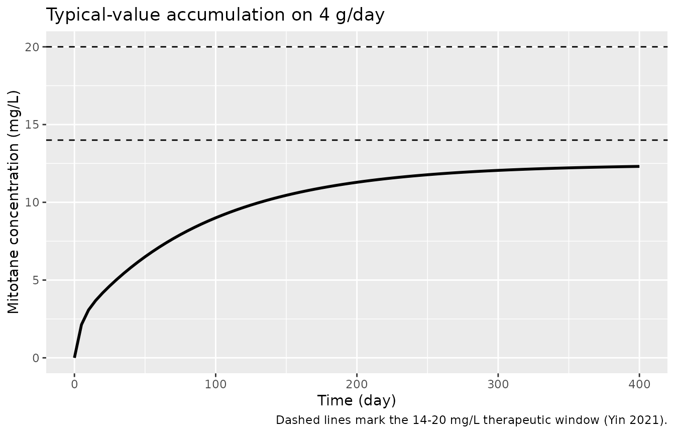
Mitotane accumulates slowly toward its 14-20 mg/L target over months of daily dosing, the central clinical challenge the paper addresses. The typical-value profile below shows a male, 80 kg, 172 cm, reference-genotype patient on a constant 4 g/day regimen.
acc <- as.data.frame(
  rxode2::et(amt = 4000, cmt = "depot", ii = 1, until = 400, addl = 400) |>
    rxode2::et(seq(0, 400, by = 5))
)
acc$WT <- 80; acc$HT <- 172; acc$SEXF <- 0; acc$OCC <- 1
acc$CYP2C19_S2_CARRIER <- 0; acc$SNP_SLCO1B3_RS7311358_G_CARRIER <- 0
acc$SNP_SLCO1B1_RS4149057_CC <- 0; acc$SNP_SLCO1B1_RS4149057_TT <- 0

acc_sim <- rxode2::rxSolve(mod, acc)
#> ℹ omega/sigma items treated as zero: 'etalcl', 'etalvc', 'etalq', 'etalvp', 'etaiov_cl_1', 'etaiov_cl_2', 'etaiov_cl_3', 'etaiov_cl_4', 'etaiov_cl_5', 'etaiov_cl_6', 'etaiov_cl_7', 'etaiov_cl_8'

ggplot(as.data.frame(acc_sim), aes(time, Cc)) +
  geom_hline(yintercept = c(14, 20), linetype = "dashed") +
  geom_line(linewidth = 1) +
  labs(
    x = "Time (day)", y = "Mitotane concentration (mg/L)",
    title = "Typical-value accumulation on 4 g/day",
    caption = "Dashed lines mark the 14-20 mg/L therapeutic window (Yin 2021)."
  )
Assumptions and deviations
- The paper does not report a conventional NCA table (Cmax / Tmax / AUC per dose group), so validation here is structural: the exact reproduction of the Table 2 genotype multipliers and covariate power terms on the typical individual, dose-proportionality of a linear model, and the cohort-median terminal half-life against the value reported in the Discussion (median 101.5 days). The maintainers judged these the faithful checks for a linear popPK model whose published evaluation was a prediction-corrected VPC and goodness-of-fit plots that require the original (non-public) data.
- Interindividual-variability and interoccasion-variability magnitudes
are encoded on the standard-deviation scale: the CV%
values printed in Table 2 are used directly as the standard deviation of
the log-normal random effect, matching the authors’ Shiny app (which
draws
rnorm(sd = CV%/100)insideexp(eta)), not as thesqrt(exp(omega^2)-1)log-normal CV. - Interoccasion variability is applied to CL/F with one occasion per
200 days of treatment. Eight occasions (
OCC1-8, covering 0-1600 days) are provided; the occasion-1 variance is estimated and occasions 2-8 repeat it (the analogue of NONMEM$OMEGA BLOCK(1) SAME). Records withOCCoutside 1-8 receive no IOV. The half-life and accumulation checks above hold a single occasion (OCC = 1), matching the individual-parameter interpretation used for the paper’s half-life summary. - Lean body weight is derived inside the model from weight, height and sex with the sex-specific Boer formula, and fat amount as weight minus lean body weight, exactly as coded in the authors’ Shiny app; weight and height carry no effect of their own. Two patients missing weight and five missing height were assigned the cohort median in the original analysis.
- The virtual cohort’s genotype frequencies (30% CYP2C19*2 carriers, 30% SLCO1B3 G carriers, all SLCO1B1 TC) are nominal illustrative values chosen by the maintainers to exercise the covariate model; the paper does not tabulate per-genotype counts, and the half-life assertion is centre-based so it does not depend on the exact frequencies.
- The cohort-median half-life assertion uses a wide, centre-based band (70-160 days) rather than the observed extremes, because the extreme of a random cohort is not reproducible across rxode2 builds or solver thread counts. The observed range brackets the paper’s reported range but is not gated.
- No correction or erratum notice was found for this article as of 2026-09-27 (checked via the publisher landing page, PubMed, EuropePMC and Crossref).