Cefazolin (Lanoiselee 2021)
Source:vignettes/articles/Lanoiselee_2021_cefazolin.Rmd
Lanoiselee_2021_cefazolin.RmdModel and source
- Citation: Lanoiselee J, Chaux R, Hodin S, Bourayou S, Gibert A, Philippot R, Molliex S, Zufferey PJ, Delavenne X, Ollier E. Population pharmacokinetic model of cefazolin in total hip arthroplasty. Sci Rep. 2021;11:19763. doi:10.1038/s41598-021-99162-7. PMCID PMC8492877. ClinicalTrials.gov NCT02252497 (PORTO study). Parameter estimates from Table 2 (Model 2, final model); covariate equation and error model from the Methods display equations.
- Description: Two-compartment population PK model for intravenous bolus cefazolin given as antibiotic prophylaxis to adults undergoing primary total hip arthroplasty (Lanoiselee 2021, n = 100 patients, 29% obese, 484 total plasma concentrations). Elimination clearance scales with CKD-EPI estimated creatinine clearance through an estimated power function centred at 80 mL/min/1.73 m^2; no body-size descriptor (total body weight, BMI, lean body weight) was retained. Log-normal between-subject variability on CL, Vc, Q and Vp with a CL-Vc correlation; proportional residual error. Estimated in Monolix 4.3 by SAEM.
- Article: https://doi.org/10.1038/s41598-021-99162-7 (open access, Sci Rep 2021;11:19763)
No supplementary material and no correction notice were found for this article (EuropePMC, checked 2026-09-29).
Population
Lanoiselee et al. analysed residual plasma from 100 adults undergoing cementless primary unilateral total hip arthroplasty at the University Hospital of Saint-Etienne, France, enrolled in the PORTO tranexamic-acid trial (NCT02252497) between April 2014 and December 2015. Mean age was 67 years (range 24-91), mean total body weight 76 kg (range 48-123), 49 were female and 29 were obese (BMI > 30 kg/m^2; 5 above 35 kg/m^2). Mean CKD-EPI creatinine clearance was 83 mL/min/1.73 m^2 (range 17-129); 8 patients were between 30 and 60 and 1 below 30 mL/min/1.73 m^2 (Table 1). Cefazolin was given as a direct intravenous bolus at anaesthesia induction: 2000 mg in 96 patients, 3000 mg in 1 and 4000 mg in 3 (dose doubled when BMI > 35 kg/m^2 and body weight > 100 kg). Samples were drawn 3 and 20 min after the bolus, at the end of surgery, and at 3 h and 8 h, giving 484 total-plasma concentrations (LC-MS/MS, LLOQ 5 mg/L).
The same information is available programmatically via
readModelDb("Lanoiselee_2021_cefazolin")()$population.
Source trace
| Equation / parameter | Value | Source location |
|---|---|---|
| Structure: two-compartment, IV bolus into central | n/a | Results, ‘Population PK model’ |
cl = exp(lcl + etalcl) * (CRCL / 80)^e_crcl_cl |
n/a | Methods covariate equation; Table 2 row ‘CL (L/h) = theta1 x (CrCL/80)^theta2’ |
lcl |
log(2.86) L/h | Table 2, Model 2, theta1 (RSE 3.26%) |
e_crcl_cl |
0.79 | Table 2, Model 2, theta2 (RSE 10.6%) |
lvc |
log(5.2) L | Table 2, Model 2, Vc (RSE 6.89%) |
lq |
log(10.9) L/h | Table 2, Model 2, Q (RSE 11.9%) |
lvp |
log(4.56) L | Table 2, Model 2, Vp (RSE 3.07%) |
etalcl |
0.32^2 = 0.1024 | Table 2, Model 2, Omega CL = 32 |
etalvc |
0.57^2 = 0.3249 | Table 2, Model 2, Omega Vc = 57 |
cov(etalcl, etalvc) |
0.83 x 0.32 x 0.57 = 0.151392 | Table 2, Model 2, correlation CL-Vc = 0.83 |
etalq |
0.66^2 = 0.4356 | Table 2, Model 2, Omega Q = 66 |
etalvp |
0.10^2 = 0.01 | Table 2, Model 2, Omega Vp = 10 |
propSd |
0.12 | Table 2, Model 2, proportional residual = 12; Methods error-model equation with a = 0 |
CRCL centring value |
80 mL/min/1.73 m^2 | Methods: ‘CrCLi is centred on 80’ |
Omega scale
Table 2 prints the random-effect rows as whole numbers (Omega CL =
32, Omega Vc = 57, …) and its footnote calls them variances. Monolix
reports each omega as the standard deviation of the
log-normal random effect, so the printed numbers could be either 100 x
SD or 100 x variance. The two readings give very different spreads (SD
0.32 versus SD 0.57 on CL), and the paper’s own Table 3 separates them:
it reports the probability that total cefazolin stays above 20 mg/L at
2.01 h and at 4 h after a 2000 mg bolus for four CrCL values. The chunk
below reproduces Table 3 under both readings.
The simulation is deterministic: the random effects are drawn with
base R and passed to the model as data (zeroRe() removes
the model’s own random effects), and the proportional residual error is
integrated analytically with pnorm(). Base R’s generator is
stable across builds and thread counts, so the numbers below are
reproducible on every machine.
mod <- readModelDb("Lanoiselee_2021_cefazolin")
ui <- rxode2::rxode(mod)
#> ℹ parameter labels from comments will be replaced by 'label()'
omega_sd <- ui$omega # the packaged (SD-reading) covariance matrix
eta_names <- colnames(omega_sd)
prop_sd <- ui$theta[["propSd"]]

# Alternative reading: the printed numbers /100 are VARIANCES, with the same
# correlation structure.
omega_var <- local({
  d <- diag(sqrt(sqrt(diag(omega_sd))))
  d %*% stats::cov2cor(omega_sd) %*% d
})
dimnames(omega_var) <- dimnames(omega_sd)

set.seed(20211006)
n_pta <- 200L
z <- matrix(rnorm(n_pta * length(eta_names)), n_pta)
crcl_levels <- c(120, 90, 60, 30)

pta_events <- function(omega, reading) {
  etas <- z %*% chol(omega)
  colnames(etas) <- eta_names
  base <- dplyr::bind_cols(tibble::tibble(sid = seq_len(n_pta)), tibble::as_tibble(etas))
  cohort <- tidyr::crossing(base, CRCL = crcl_levels) |>
    dplyr::mutate(id = dplyr::row_number(), reading = reading)
  dplyr::bind_rows(
    cohort |> dplyr::mutate(time = 0, evid = 1L, amt = 2000, cmt = "central"),
    cohort |> dplyr::mutate(time = 2.01, evid = 0L, amt = 0, cmt = "central"),
    cohort |> dplyr::mutate(time = 4, evid = 0L, amt = 0, cmt = "central")
  ) |>
    dplyr::arrange(id, time, dplyr::desc(evid))
}

solve_with_data_etas <- function(ev) {
  withCallingHandlers(
    rxode2::rxSolve(rxode2::zeroRe(mod), events = ev, keep = c("CRCL", "reading")),
    warning = function(w) {
      if (grepl("without 'omega'", conditionMessage(w), fixed = TRUE)) {
        invokeRestart("muffleWarning")
      }
    }
  )
}

pta_sim <- dplyr::bind_rows(
  as.data.frame(solve_with_data_etas(pta_events(omega_sd, "SD (packaged)"))),
  as.data.frame(solve_with_data_etas(pta_events(omega_var, "variance")))
)
#> ℹ parameter labels from comments will be replaced by 'label()'
#> ℹ omega/sigma items treated as zero: 'etalcl', 'etalvc', 'etalq', 'etalvp'
#> ℹ parameter labels from comments will be replaced by 'label()'
#> ℹ omega/sigma items treated as zero: 'etalcl', 'etalvc', 'etalq', 'etalvp'
stopifnot(nrow(pta_sim) == 2L * 2L * n_pta * length(crcl_levels))

pta_tab <- pta_sim |>
  dplyr::group_by(reading, CRCL, time) |>
  dplyr::summarise(
    pta_ipred = 100 * mean(Cc > 20),
    pta_obs = 100 * mean(stats::pnorm(20, Cc, prop_sd * Cc, lower.tail = FALSE)),
    .groups = "drop"
  )

published_pta <- tibble::tribble(
  ~CRCL, ~time, ~pta_published,
  120, 2.01, 100,
  90, 2.01, 100,
  60, 2.01, 100,
  30, 2.01, 100,
  120, 4, 94.5,
  90, 4, 99.8,
  60, 4, 100,
  30, 4, 100
)

pta_cmp <- dplyr::inner_join(pta_tab, published_pta, by = c("CRCL", "time"))
stopifnot(nrow(pta_cmp) == 16L)

pta_cmp |>
  dplyr::arrange(reading, dplyr::desc(CRCL), time) |>
  dplyr::mutate(time = sprintf("%.2f", time)) |>
  dplyr::rename(
    "Omega reading" = reading,
    "CrCL (mL/min/1.73 m^2)" = CRCL,
    "Time (h)" = time,
    "PTA, no residual (%)" = pta_ipred,
    "PTA, with residual (%)" = pta_obs,
    "Published PTA (%)" = pta_published
  ) |>
knitr::kable(digits = 1, caption = "Replicates Table 3 of Lanoiselee 2021: probability of total cefazolin > 20 mg/L after a 2000 mg bolus.")| Omega reading | CrCL (mL/min/1.73 m^2) | Time (h) | PTA, no residual (%) | PTA, with residual (%) | Published PTA (%) |
|---|---|---|---|---|---|
| SD (packaged) | 120 | 2.01 | 100.0 | 100.0 | 100.0 |
| SD (packaged) | 120 | 4.00 | 94.0 | 93.9 | 94.5 |
| SD (packaged) | 90 | 2.01 | 100.0 | 100.0 | 100.0 |
| SD (packaged) | 90 | 4.00 | 98.5 | 98.5 | 99.8 |
| SD (packaged) | 60 | 2.01 | 100.0 | 100.0 | 100.0 |
| SD (packaged) | 60 | 4.00 | 100.0 | 100.0 | 100.0 |
| SD (packaged) | 30 | 2.01 | 100.0 | 100.0 | 100.0 |
| SD (packaged) | 30 | 4.00 | 100.0 | 100.0 | 100.0 |
| variance | 120 | 2.01 | 98.5 | 98.3 | 100.0 |
| variance | 120 | 4.00 | 78.5 | 77.5 | 94.5 |
| variance | 90 | 2.01 | 99.0 | 98.8 | 100.0 |
| variance | 90 | 4.00 | 91.0 | 90.3 | 99.8 |
| variance | 60 | 2.01 | 100.0 | 99.8 | 100.0 |
| variance | 60 | 4.00 | 98.0 | 97.7 | 100.0 |
| variance | 30 | 2.01 | 100.0 | 100.0 | 100.0 |
| variance | 30 | 4.00 | 99.0 | 99.4 | 100.0 |
pta_cell <- function(rd, crcl, t) {
  v <- pta_cmp$pta_obs[pta_cmp$reading == rd & pta_cmp$CRCL == crcl & pta_cmp$time == t]
  if (length(v) != 1L) stop("no unique PTA row for ", rd, " / ", crcl, " / ", t)
  v
}
stopifnot(
  # SD reading reproduces every Table 3 cell within 3 percentage points.
  all(abs(pta_cmp$pta_obs - pta_cmp$pta_published)[pta_cmp$reading == "SD (packaged)"] < 3),
  # Mutation control: the variance reading misses the CrCL 120 and 90 cells
  # at 4 h by far more than that, so this table does discriminate the scale.
  pta_cell("variance", 120, 4) < 94.5 - 8,
  pta_cell("variance", 90, 4) < 99.8 - 4
)
Under the SD reading every Table 3 cell is reproduced within 3
percentage points (published 94.5% and 99.8% at 4 h for CrCL 120 and 90
against 93.9% and 98.5% here; 100% elsewhere). Under the variance
reading the 4 h values at CrCL 120 and 90 fall to 77.5% and 90.3%. The
packaged model therefore uses the printed values as 100 x SD, and the
proportional residual error (printed 12) is read on the same scale as
propSd = 0.12.
Typical-value checks
A deterministic typical-value solve at the four CrCL values of Figure 4 is compared with the closed-form two-compartment bolus solution.
t_grid <- sort(unique(c(seq(0, 1, by = 0.05), seq(1, 24, by = 0.25), 2.01)))
typ_events <- tidyr::crossing(id = seq_along(crcl_levels), time = t_grid) |>
  dplyr::mutate(evid = 0L, amt = 0) |>
  dplyr::bind_rows(tibble::tibble(id = seq_along(crcl_levels), time = 0, evid = 1L, amt = 2000)) |>
  dplyr::mutate(cmt = "central", CRCL = crcl_levels[id]) |>
  dplyr::arrange(id, time, dplyr::desc(evid))

typ <- rxode2::rxSolve(rxode2::zeroRe(mod), events = typ_events, keep = "CRCL",
                       rtol = 1e-10, atol = 1e-12) |>
  as.data.frame()
#> ℹ parameter labels from comments will be replaced by 'label()'
#> ℹ omega/sigma items treated as zero: 'etalcl', 'etalvc', 'etalq', 'etalvp'
#> Warning: multi-subject simulation without without 'omega'

th <- ui$theta
closed_form <- function(t, dose, cl, vc, q, vp) {
  k10 <- cl / vc; k12 <- q / vc; k21 <- q / vp
  s <- k10 + k12 + k21
  r <- sqrt(s^2 - 4 * k10 * k21)
  a <- (s + r) / 2; b <- (s - r) / 2
  dose / vc * ((a - k21) / (a - b) * exp(-a * t) + (k21 - b) / (a - b) * exp(-b * t))
}
typ <- typ |>
  dplyr::mutate(
    cl_typ = exp(th[["lcl"]]) * (CRCL / 80)^th[["e_crcl_cl"]],
    Cc_cf = closed_form(time, 2000, cl_typ, exp(th[["lvc"]]), exp(th[["lq"]]), exp(th[["lvp"]]))
  )
rel_err <- max(abs(typ$Cc / typ$Cc_cf - 1))
stopifnot(rel_err < 1e-6)
rel_err
#> [1] 7.166894e-10
The ODE solution matches the closed form to a maximum relative error of 7.2^{-10}.
Replicate Figure 4
Figure 4 shows the concentration-time course after a 2000 mg bolus at CrCL 30, 60, 90 and 120 mL/min/1.73 m^2, with the typical profile, an interpatient variability band and the 20 and 360 mg/L thresholds. The stochastic cohort below uses 200 virtual patients per CrCL level.
rxode2::rxSetSeed(20211006)
n_sub <- 200L
vpc_times <- sort(unique(c(0, 3 / 60, 20 / 60, seq(0.25, 8, by = 0.25))))
vpc_events <- tidyr::crossing(sid = seq_len(n_sub), CRCL = crcl_levels) |>
  dplyr::mutate(id = dplyr::row_number())
vpc_events <- dplyr::bind_rows(
  vpc_events |> dplyr::mutate(time = 0, evid = 1L, amt = 2000),
  tidyr::crossing(vpc_events, time = vpc_times) |> dplyr::mutate(evid = 0L, amt = 0)
) |>
  dplyr::mutate(cmt = "central") |>
  dplyr::arrange(id, time, dplyr::desc(evid))
stopifnot(dplyr::n_distinct(vpc_events$id) == n_sub * length(crcl_levels))

vpc <- rxode2::rxSolve(mod, events = vpc_events, keep = "CRCL") |> as.data.frame()
#> ℹ parameter labels from comments will be replaced by 'label()'
band <- vpc |>
  dplyr::filter(time > 0) |>
  dplyr::group_by(CRCL, time) |>
  dplyr::summarise(
    lo = quantile(ipredSim, 0.05), hi = quantile(ipredSim, 0.95),
    .groups = "drop"
  )
typ_plot <- typ |> dplyr::filter(time > 0, time <= 8)

ggplot() +
  geom_ribbon(data = band, aes(time, ymin = lo, ymax = hi), fill = "steelblue", alpha = 0.3) +
  geom_line(data = typ_plot, aes(time, Cc)) +
  geom_hline(yintercept = c(20, 360), linetype = "dashed", colour = "red") +
  facet_wrap(~ paste("CrCL", CRCL, "mL/min/1.73 m^2"), nrow = 1) +
  scale_y_log10() +
  labs(
    x = "Time after bolus (h)", y = "Total cefazolin (mg/L)",
    caption = "Replicates Figure 4 of Lanoiselee 2021. Line: typical value; band: 5th-95th percentile of individual predictions."
  )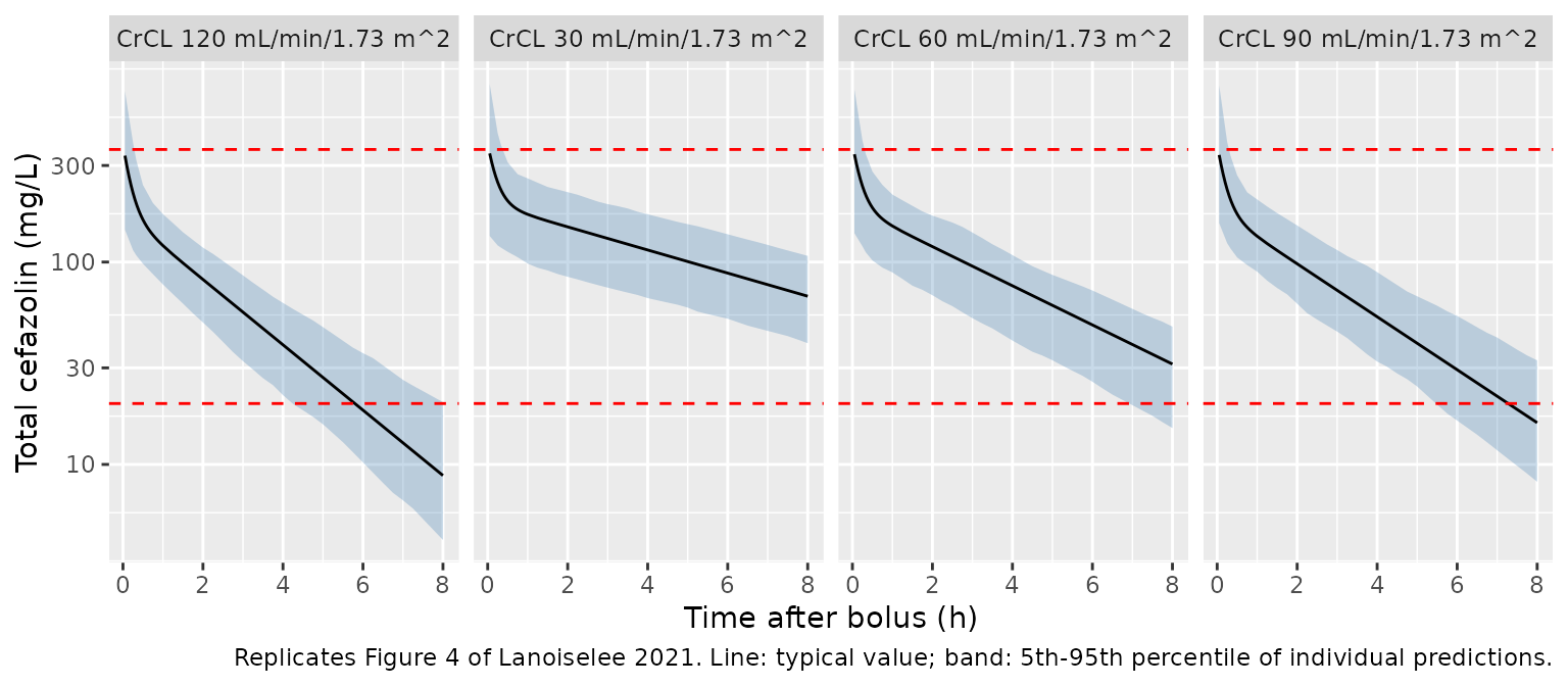
The paper states that after a 2000 mg bolus concentrations stay above 20 mg/L throughout surgery regardless of renal function. The typical-value concentration at the mean time of skin closure (2.01 h) and at 4 h is shown below; the lowest value, at CrCL 120, is still above the threshold at 4 h.
typ_at <- typ |>
  dplyr::filter(abs(time - 0.05) < 1e-9 | abs(time - 2.01) < 1e-9 | abs(time - 4) < 1e-9) |>
  dplyr::mutate(time = round(time, 2)) |>
  dplyr::select(CRCL, time, Cc) |>
  tidyr::pivot_wider(names_from = time, values_from = Cc, names_prefix = "t_")
stopifnot(nrow(typ_at) == 4L, all(typ_at$t_4 > 20))
typ_at |>
  dplyr::rename(
    "CrCL (mL/min/1.73 m^2)" = CRCL,
    "Cc at 3 min (mg/L)" = t_0.05,
    "Cc at 2.01 h (mg/L)" = t_2.01,
    "Cc at 4 h (mg/L)" = t_4
  ) |>
knitr::kable(digits = 1, caption = "Typical total cefazolin concentrations after a 2000 mg bolus.")| CrCL (mL/min/1.73 m^2) | Cc at 3 min (mg/L) | Cc at 2.01 h (mg/L) | Cc at 4 h (mg/L) |
|---|---|---|---|
| 120 | 335.6 | 81.7 | 39.0 |
| 90 | 338.2 | 97.7 | 53.6 |
| 60 | 341.0 | 119.0 | 76.4 |
| 30 | 344.1 | 149.0 | 114.7 |
Figure 5 regimens (illustrative)
Figure 5 compares a 4000 mg bolus followed by 2000 mg at 4 h with a 2000 mg bolus followed by 1000 mg at 4 h in the five patients with BMI > 35 kg/m^2 and body weight > 100 kg. Those curves use the patients’ individual (post hoc) parameters, which are not published, so they cannot be reproduced. The chunk below shows the same two regimens for a typical patient at the centring CrCL of 80 mL/min/1.73 m^2. Because the model is linear, the higher regimen is exactly twice the lower one.
reg_events <- dplyr::bind_rows(
  tibble::tibble(id = 1L, regimen = "2000 mg + 1000 mg at 4 h", time = c(0, 4), amt = c(2000, 1000)),
  tibble::tibble(id = 2L, regimen = "4000 mg + 2000 mg at 4 h", time = c(0, 4), amt = c(4000, 2000))
) |>
  dplyr::mutate(evid = 1L)
reg_events <- dplyr::bind_rows(
  reg_events,
  tidyr::crossing(dplyr::distinct(reg_events, id, regimen), time = seq(0.05, 8, by = 0.05)) |>
    dplyr::mutate(evid = 0L, amt = 0)
) |>
  dplyr::mutate(cmt = "central", CRCL = 80) |>
  dplyr::arrange(id, time, dplyr::desc(evid))

reg <- rxode2::rxSolve(rxode2::zeroRe(mod), events = reg_events, keep = "regimen",
                       rtol = 1e-10, atol = 1e-12) |>
  as.data.frame()
#> ℹ parameter labels from comments will be replaced by 'label()'
#> ℹ omega/sigma items treated as zero: 'etalcl', 'etalvc', 'etalq', 'etalvp'
#> Warning: multi-subject simulation without without 'omega'
ratio <- reg$Cc[reg$id == 2] / reg$Cc[reg$id == 1]
stopifnot(length(ratio) > 0, max(abs(ratio / 2 - 1)) < 1e-6)

ggplot(reg, aes(time, Cc, colour = regimen)) +
  geom_line() +
  geom_hline(yintercept = c(20, 360), linetype = "dashed", colour = "red") +
  scale_y_log10() +
  labs(x = "Time after first bolus (h)", y = "Total cefazolin (mg/L)", colour = NULL,
       caption = "Typical patient, CrCL 80 mL/min/1.73 m^2 (cf. Figure 5 of Lanoiselee 2021).") +
  theme(legend.position = "bottom")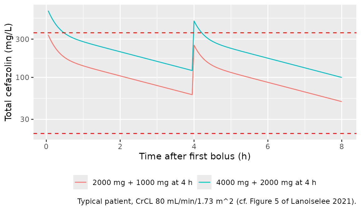
PKNCA validation
The paper reports no NCA table. PKNCA is run on the stochastic Figure
4 cohort, extended to 48 h so the terminal phase is captured, and each
subject’s AUC0-inf is checked against
Dose / CL_i using that subject’s own simulated
clearance.
nca_times <- sort(unique(c(0, 3 / 60, 20 / 60, seq(0.25, 2, by = 0.25), seq(2.5, 12, by = 0.5), seq(13, 48, by = 1))))
nca_ev <- tidyr::crossing(sid = seq_len(n_sub), CRCL = crcl_levels) |>
  dplyr::mutate(id = dplyr::row_number(), treatment = paste0("CrCL ", CRCL))
nca_ev <- dplyr::bind_rows(
  nca_ev |> dplyr::mutate(time = 0, evid = 1L, amt = 2000),
  tidyr::crossing(nca_ev, time = nca_times) |> dplyr::mutate(evid = 0L, amt = 0)
) |>
  dplyr::mutate(cmt = "central") |>
  dplyr::arrange(id, time, dplyr::desc(evid))

nca_sim <- rxode2::rxSolve(mod, events = nca_ev, keep = c("CRCL", "treatment")) |>
  as.data.frame()
stopifnot(all(nca_sim$ipredSim >= -1e-6 * max(nca_sim$ipredSim)))

conc_df <- nca_sim |>
  dplyr::filter(!is.na(ipredSim)) |>
  dplyr::transmute(id, time, treatment, Cc = pmax(ipredSim, 0))
dose_df <- nca_ev |>
  dplyr::filter(evid == 1) |>
  dplyr::select(id, time, amt, treatment)

conc_obj <- PKNCA::PKNCAconc(conc_df, Cc ~ time | treatment + id)
dose_obj <- PKNCA::PKNCAdose(dose_df, amt ~ time | treatment + id)
intervals <- data.frame(start = 0, end = Inf, cmax = TRUE, aucinf.obs = TRUE, half.life = TRUE)
nca_res <- PKNCA::pk.nca(PKNCA::PKNCAdata(conc_obj, dose_obj, intervals = intervals))

nca_ind <- as.data.frame(nca_res) |>
  dplyr::filter(PPTESTCD %in% c("cmax", "aucinf.obs", "half.life")) |>
  dplyr::select(id, treatment, PPTESTCD, PPORRES) |>
  tidyr::pivot_wider(names_from = PPTESTCD, values_from = PPORRES) |>
  dplyr::left_join(dplyr::distinct(nca_sim, id, cl, vc), by = "id") |>
  dplyr::mutate(
    pct_diff = 100 * (aucinf.obs / (2000 / cl) - 1),
    cmax_diff = 100 * (cmax / (2000 / vc) - 1)
  )
stopifnot(nrow(nca_ind) == n_sub * length(crcl_levels))
stopifnot(
  abs(median(nca_ind$pct_diff)) < 1,
  quantile(abs(nca_ind$pct_diff), 0.9) < 3,
  # Time-zero record follows the bolus, so Cmax is the instantaneous Dose/Vc.
  max(abs(nca_ind$cmax_diff)) < 1e-3
)

nca_ind |>
  dplyr::group_by(treatment) |>
  dplyr::summarise(
    cmax = median(cmax), aucinf = median(aucinf.obs), t_half = median(half.life),
    auc_vs_dose_cl = median(pct_diff), .groups = "drop"
  ) |>
  dplyr::arrange(dplyr::desc(as.numeric(sub("CrCL ", "", treatment)))) |>
  dplyr::rename(
    "Group" = treatment,
    "Median Cmax (mg/L)" = cmax,
    "Median AUC0-inf (mg*h/L)" = aucinf,
    "Median terminal t1/2 (h)" = t_half,
    "Median AUC0-inf vs Dose/CL (%)" = auc_vs_dose_cl
  ) |>
knitr::kable(digits = 1, caption = "PKNCA summary of the simulated 2000 mg bolus cohort (200 patients per CrCL level).")| Group | Median Cmax (mg/L) | Median AUC0-inf (mg*h/L) | Median terminal t1/2 (h) | Median AUC0-inf vs Dose/CL (%) |
|---|---|---|---|---|
| CrCL 120 | 411.6 | 521.2 | 2.0 | 0.3 |
| CrCL 90 | 390.1 | 662.0 | 2.4 | 0.2 |
| CrCL 60 | 358.8 | 832.7 | 3.3 | 0.1 |
| CrCL 30 | 354.0 | 1500.7 | 5.7 | 0.1 |
AUC0-inf agrees with Dose / CL_i subject by
subject (median difference below 1%), confirming dose, clearance and
units are consistent. Because the time-zero record is taken after the
bolus, PKNCA’s Cmax equals each subject’s instantaneous
Dose / Vc.
Assumptions and deviations
-
Omega and residual-error scale. Table 2 labels the
random-effect rows as variances, but the printed numbers are 100 x the
Monolix log-scale SD. The maintainers settled this against the paper’s
own Table 3 PTA values (see “Omega scale” above). The proportional
residual error printed as 12 is taken as
propSd = 0.12on the same basis; Table 3 is not sensitive enough to test it separately. -
CrCL units. Table 1, Table 3 and the Figure 4
caption give CKD-EPI CrCL in mL/min/1.73 m^2, the native CKD-EPI unit,
while the Table 2 and Table 3 footnotes say mL/min. The model uses the
BSA-normalized
CRCLcovariate. - Residual error in Table 3. The paper does not say whether its PTA was computed on individual predictions or on simulated observations; both are shown and differ by at most 1 percentage points.
- Figure 5 uses individual post hoc parameters that are not published; the regimens are shown for a typical patient only.
-
Covariates tested but not retained (age, total body
weight, BMI, lean body weight and sex) are recorded in the model’s
covariatesDataExcludedmetadata. Cockcroft-Gault CrCL, tested as an alternative renal-function estimator to CKD-EPI, is noted in theCRCLcovariate entry.