Gottingen minipig mAb IV+SC PK panel (Zheng 2012)
Source:vignettes/articles/Zheng_2012_minipig_mab.Rmd
Zheng_2012_minipig_mab.RmdPaper and source
- Citation: Zheng Y, Tesar DB, Benincosa L, Birnbock H, Boswell CA, Bumbaca D, Cowan KJ, Danilenko DM, Daugherty AL, Fielder PJ, Grimm HP, Joshi A, Justies N, Kolaitis G, Lewin-Koh N, Li J, McVay S, O’Mahony J, Otteneder M, Pantze M, Putnam WS, Qiu ZJ, Ruppel J, Singer T, Stauch O, Theil FP, Visich J, Yang J, Ying Y, Khawli LA, et al. Minipig as a potential translatable model for monoclonal antibody pharmacokinetics after intravenous and subcutaneous administration. MAbs. 2012;4(2):243-255. doi:10.4161/mabs.4.2.19387.
- Article: https://doi.org/10.4161/mabs.4.2.19387
- PMID: 22453096
This vignette is a joint validation of the nine minipig popPK models packaged from Zheng 2012 – one per antibody tested in the study. The paper reports population-mean IV and SC pharmacokinetics of nine IgGs (eight non-disclosed humanized IgG1 / stabilized IgG4 antibodies labelled mAb1..mAb8 plus commercial adalimumab) in Gottingen minipigs across four contract research organisations.
Each mAb was fit independently to a two-compartment model with
first-order SC absorption and linear central clearance (paper Eq. 1).
mAb7 has an additional saturable (Michaelis-Menten) elimination arm
(paper Eq. 2). mAb8 was studied by IV only, so it carries no SC
absorption or bioavailability. In line with the standing “replicate the
author’s modelling structure” policy this yields nine .R
files, one per antibody, sharing this single vignette.
model_names <- c(
  "Zheng_2012_mAb1_minipig",
  "Zheng_2012_mAb2_minipig",
  "Zheng_2012_mAb3_minipig",
  "Zheng_2012_mAb4_minipig",
  "Zheng_2012_mAb5_minipig",
  "Zheng_2012_mAb6_minipig",
  "Zheng_2012_mAb7_minipig",
  "Zheng_2012_mAb8_minipig",
  "Zheng_2012_adalimumab_minipig"
)
mods <- setNames(lapply(model_names, readModelDb), sub("_minipig$", "", sub("^Zheng_2012_", "", model_names)))
Population
Zheng 2012 pooled nine independent IV+SC single-dose studies in Gottingen minipigs (male or female, 8-11 kg, aged for acclimation for 15-20 days before study). Studies were run across four CROs (Pipeline Biotech / Denmark, Charles Rivers Labs / Ohio, Covance / Harrogate, LAB Research / Denmark). Each mAb was dosed to three to five animals per IV or SC arm. IV administration was a single bolus via jugular cannula or ear-vein catheter; SC administration was in either the scapular or inguinal region depending on the mAb (Table 5). Blood samples were drawn from pre-dose through Day 28 post-dose.
Per Table 4, the antibodies span a wide pI range (6.1 for mAb1 up to 9.4 for mAb5). Their FcRn-binding affinities to porcine, human and cynomolgus monkey FcRn are all in the same range (280-550 nM, Table 4), confirming that non-FcRn-dependent mechanisms drive the observed PK differences between mAbs.
The per-antibody population metadata (n_subjects, mean
body weights, dose, administration site) is preserved on each model file
– for example
readModelDb("Zheng_2012_mAb1_minipig")()$population.
Source trace
Every model parameter is sourced from Table 1 of Zheng 2012
(population-mean estimates); minipig study details are from Table 5, and
pI / FcRn KD are from Table 4. The in-file comments next to each
ini() entry give a per-parameter row-level pointer.
tbl1 <- tibble::tribble(
  ~mAb,          ~pI,   ~CL_mL_day_kg, ~Q_mL_day_kg, ~Vc_mL_kg, ~Vp_mL_kg, ~T12beta_days, ~Ka_1_day, ~F_pct,       ~Tmax_days,
  "mAb1",        6.1,   2.83,          128,          51.9,      54.6,      26.2,           1.02,      97.5,         4,
  "mAb2",        8.7,   36.4,          24.2,         56.4,      134,       6.86,           0.316,     79.9,         2,
  "mAb3",        9.1,   4.48,          72.5,         36.6,      70.9,      17.1,           0.635,     65.8,         2,
  "mAb4",        9.3,   11.1,          199,          47.3,      97.8,      9.29,           1.61,      36.3,         2,
  "mAb5",        9.4,   6.07,          16.0,         44.7,      37.0,      10.1,           0.862,     81.2,         2,
  "mAb6",        9.2,   8.06,          10.2,         58.5,      26.0,      7.91,           0.530,     68.9,         2,
  "mAb7",        8.9,   5.06,          17.6,         61.6,      37.4,      NA_real_,       0.828,     85.4,         3,
  "mAb8",        8.7,   2.45,          27.6,         36.0,      36.4,      20.9,           NA_real_,  NA_real_,     NA_real_,
  "adalimumab",  8.8,   3.48,          24.0,         55.4,      13.5,      13.8,           4.61,      82.9,         1
)
tbl1 |>
  dplyr::rename(
    "mAb"              = mAb,
    "pI"               = pI,
    "CL (mL/day/kg)"   = CL_mL_day_kg,
    "Q (mL/day/kg)"    = Q_mL_day_kg,
    "Vc (mL/kg)"       = Vc_mL_kg,
    "Vp (mL/kg)"       = Vp_mL_kg,
    "T1/2 beta (days)" = T12beta_days,
    "Ka (1/day)"       = Ka_1_day,
    "F (%)"            = F_pct,
    "Tmax (days)"      = Tmax_days
  ) |>
  knitr::kable(
    caption = "Zheng 2012 Table 1 (population mean PK parameters) with Table 4 pI; used as the source trace for the packaged models. mAb7 additionally has nonlinear Vmax = 165 ug/day/kg and Km = 8.27 ug/mL (Table 1 footnote g). mAb7 T1/2beta and mAb8 SC parameters are not reported."
)| mAb | pI | CL (mL/day/kg) | Q (mL/day/kg) | Vc (mL/kg) | Vp (mL/kg) | T1/2 beta (days) | Ka (1/day) | F (%) | Tmax (days) |
|---|---|---|---|---|---|---|---|---|---|
| mAb1 | 6.1 | 2.83 | 128.0 | 51.9 | 54.6 | 26.20 | 1.020 | 97.5 | 4 |
| mAb2 | 8.7 | 36.40 | 24.2 | 56.4 | 134.0 | 6.86 | 0.316 | 79.9 | 2 |
| mAb3 | 9.1 | 4.48 | 72.5 | 36.6 | 70.9 | 17.10 | 0.635 | 65.8 | 2 |
| mAb4 | 9.3 | 11.10 | 199.0 | 47.3 | 97.8 | 9.29 | 1.610 | 36.3 | 2 |
| mAb5 | 9.4 | 6.07 | 16.0 | 44.7 | 37.0 | 10.10 | 0.862 | 81.2 | 2 |
| mAb6 | 9.2 | 8.06 | 10.2 | 58.5 | 26.0 | 7.91 | 0.530 | 68.9 | 2 |
| mAb7 | 8.9 | 5.06 | 17.6 | 61.6 | 37.4 | NA | 0.828 | 85.4 | 3 |
| mAb8 | 8.7 | 2.45 | 27.6 | 36.0 | 36.4 | 20.90 | NA | NA | NA |
| adalimumab | 8.8 | 3.48 | 24.0 | 55.4 | 13.5 | 13.80 | 4.610 | 82.9 | 1 |
Study-design details per Table 5:
tbl5 <- tibble::tribble(
  ~mAb,          ~IV_weight_kg, ~IV_dose_per_kg, ~SC_weight_kg, ~SC_dose_per_kg, ~SC_site,
  "mAb1",        9.4,  "5 mg/kg IV",  9.9,  "5 mg/kg SC",              "scapular",
  "mAb2",        9.5,  "5 mg/kg IV",  9.7,  "5 mg/kg SC",              "scapular",
  "mAb3",        8.2,  "5 mg/kg IV",  8.3,  "5 mg/kg SC",              "scapular",
  "mAb4",        8.4,  "5 mg/kg IV",  8.4,  "5 mg/kg SC",              "scapular",
  "mAb5",        9.1,  "20 mg/kg IV", 8.9,  "180 mg SC (20.2 mg/kg)",  "inguinal",
  "mAb6",        8.9,  "10 mg/kg IV", 8.6,  "120 mg SC (13.95 mg/kg)", "inguinal",
  "mAb7",        8.4,  "9 mg/kg IV",  8.2,  "108 mg SC (13.17 mg/kg)", "inguinal",
  "mAb8",        9.7,  "10 mg/kg IV", NA,   "not conducted",           "-",
  "adalimumab",  10.2, "40 mg (3.92 mg/kg) IV", 10.0, "40 mg SC (4.00 mg/kg)", "inguinal"
)
tbl5 |>
  dplyr::rename(
    "mAb"                        = mAb,
    "IV mean body weight (kg)"   = IV_weight_kg,
    "IV dose"                    = IV_dose_per_kg,
    "SC mean body weight (kg)"   = SC_weight_kg,
    "SC dose"                    = SC_dose_per_kg,
    "SC site"                    = SC_site
  ) |>
knitr::kable(caption = "Zheng 2012 Table 5 minipig dosing details.")| mAb | IV mean body weight (kg) | IV dose | SC mean body weight (kg) | SC dose | SC site |
|---|---|---|---|---|---|
| mAb1 | 9.4 | 5 mg/kg IV | 9.9 | 5 mg/kg SC | scapular |
| mAb2 | 9.5 | 5 mg/kg IV | 9.7 | 5 mg/kg SC | scapular |
| mAb3 | 8.2 | 5 mg/kg IV | 8.3 | 5 mg/kg SC | scapular |
| mAb4 | 8.4 | 5 mg/kg IV | 8.4 | 5 mg/kg SC | scapular |
| mAb5 | 9.1 | 20 mg/kg IV | 8.9 | 180 mg SC (20.2 mg/kg) | inguinal |
| mAb6 | 8.9 | 10 mg/kg IV | 8.6 | 120 mg SC (13.95 mg/kg) | inguinal |
| mAb7 | 8.4 | 9 mg/kg IV | 8.2 | 108 mg SC (13.17 mg/kg) | inguinal |
| mAb8 | 9.7 | 10 mg/kg IV | NA | not conducted | - |
| adalimumab | 10.2 | 40 mg (3.92 mg/kg) IV | 10.0 | 40 mg SC (4.00 mg/kg) | inguinal |
Virtual cohort and simulation
Zheng 2012 reports population-mean estimates and standard error of
the mean, but not the inter-individual variability magnitudes
(log-normal IIV was assumed in fitting) nor the proportional / additive
residual error magnitudes. The packaged models therefore encode typical
population values only (no eta* blocks, no residual error)
– deterministic single-trajectory simulations per mAb are the intended
use. See the Assumptions and deviations section.
Doses per Table 5 are entered on a per-kg basis. IV bolus doses go to
central; SC doses go to depot and are
attenuated by the fitted bioavailability F via
f(depot).
obs_times <- sort(unique(c(seq(0, 1, by = 0.05),
                           seq(1, 7, by = 0.25),
                           seq(7, 28, by = 0.5))))

# Table 5 dosing (per-kg for consistency across mAbs; SC values converted from
# total mg / mean body weight for mAb5-7 and adalimumab)
dosing <- tibble::tribble(
  ~mAb,          ~iv_mg_per_kg, ~sc_mg_per_kg,
  "mAb1",        5,             5,
  "mAb2",        5,             5,
  "mAb3",        5,             5,
  "mAb4",        5,             5,
  "mAb5",        20,            20.22,   # 180 mg / 8.9 kg
  "mAb6",        10,            13.95,   # 120 mg / 8.6 kg
  "mAb7",        9,             13.17,   # 108 mg / 8.2 kg
  "mAb8",        10,            NA_real_,
  "adalimumab",  3.92,          4.00     # 40 mg / 10.2 kg IV; 40 mg / 10.0 kg SC
)

# One "id" per (mAb, route) combination; ids are disjoint integers so bind_rows
# never merges subjects. Because each rxSolve() below has a single id, rxode2
# drops the id column from the returned data frame; we add it back manually.
# The route indicator is named `arm` (not `route`) because PKNCA reserves the
# name `route` for its automatic IV / extravascular detection.
simulate_mab <- function(mab_name, iv_dose, sc_dose, id_iv, id_sc) {
  mod  <- rxode2::rxode2(mods[[mab_name]])

  # IV arm -- dose into central compartment
  ev_iv <- rxode2::et(amt = iv_dose, cmt = "central", id = id_iv) |>
    rxode2::et(time = obs_times, id = id_iv)
  sim_iv <- as.data.frame(rxode2::rxSolve(mod, ev_iv))
  sim_iv$id  <- id_iv
  sim_iv$mAb <- mab_name
  sim_iv$arm <- "IV"

  # SC arm -- dose into depot (skip if no SC data was reported)
  if (!is.na(sc_dose)) {
    ev_sc <- rxode2::et(amt = sc_dose, cmt = "depot", id = id_sc) |>
      rxode2::et(time = obs_times, id = id_sc)
    sim_sc <- as.data.frame(rxode2::rxSolve(mod, ev_sc))
    sim_sc$id  <- id_sc
    sim_sc$mAb <- mab_name
    sim_sc$arm <- "SC"
    return(dplyr::bind_rows(sim_iv, sim_sc))
  }
  sim_iv
}

sim_list <- vector("list", nrow(dosing))
id_counter <- 1L
for (i in seq_len(nrow(dosing))) {
  id_iv <- id_counter
  id_sc <- id_counter + 1L
  id_counter <- id_counter + 2L
  sim_list[[i]] <- simulate_mab(
    mab_name = dosing$mAb[i],
    iv_dose  = dosing$iv_mg_per_kg[i],
    sc_dose  = dosing$sc_mg_per_kg[i],
    id_iv    = id_iv,
    id_sc    = id_sc
  )
}
sim <- dplyr::bind_rows(sim_list)
sim$mAb <- factor(sim$mAb, levels = dosing$mAb)
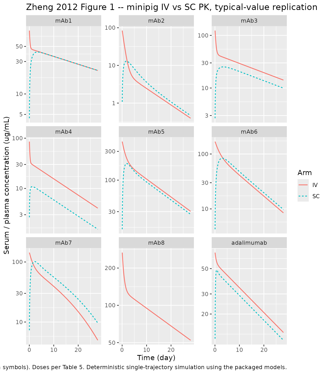
Replicate Figure 1 – concentration-time curves after IV and SC dosing
sim |>
  dplyr::filter(time > 0, Cc > 0) |>
  ggplot2::ggplot(ggplot2::aes(time, Cc, colour = arm, linetype = arm)) +
  ggplot2::geom_line(linewidth = 0.6) +
  ggplot2::scale_y_log10() +
  ggplot2::facet_wrap(~ mAb, ncol = 3, scales = "free_y") +
  ggplot2::labs(
    x = "Time (day)",
    y = "Serum / plasma concentration (ug/mL)",
    colour = "Arm", linetype = "Arm",
    title = "Zheng 2012 Figure 1 -- minipig IV vs SC PK, typical-value replication",
    caption = "Replicates the shape of Zheng 2012 Figure 1 (IV closed symbols; SC open symbols). Doses per Table 5. Deterministic single-trajectory simulation using the packaged models."
  )
PKNCA validation
Non-compartmental analysis is run per (mAb x route) group. Simulated Cmax, Tmax, AUC0-inf and terminal half-life are computed from the deterministic trajectory and then compared against the corresponding Table 1 published values.
# The concentration frame: one Cc per (id, time). Cc = 0 at time 0 is correct
# for SC (empty depot) and also correct for the deterministic IV output at t = 0
# because rxSolve returns the pre-dose zero row.
sim_nca <- sim |>
  dplyr::filter(!is.na(Cc)) |>
  dplyr::transmute(id = id, time = time, conc = Cc, mAb = as.character(mAb), arm = arm)

# Guarantee a time = 0 row per (id) with conc = 0 (correct for both IV and SC
# because rxSolve's t = 0 output is already 0 -- the row may nevertheless be
# absent when obs_times starts strictly above 0, so this guards the general
# case).
sim_nca <- dplyr::bind_rows(
  sim_nca,
  sim_nca |> dplyr::distinct(id, mAb, arm) |> dplyr::mutate(time = 0, conc = 0)
) |>
  dplyr::distinct(id, time, .keep_all = TRUE) |>
  dplyr::arrange(id, time)

# Build the dose frame directly from the dosing table so we have amt and arm
# alongside id. (The route indicator is `arm`, not `route`; PKNCA reserves
# `route` for its own IV / extravascular detection.)
dose_rows <- list()
id_counter <- 1L
for (i in seq_len(nrow(dosing))) {
  dose_rows[[length(dose_rows) + 1L]] <- tibble::tibble(
    id  = id_counter,
    time = 0,
    amt = dosing$iv_mg_per_kg[i],
    mAb = dosing$mAb[i],
    arm = "IV"
  )
  if (!is.na(dosing$sc_mg_per_kg[i])) {
    dose_rows[[length(dose_rows) + 1L]] <- tibble::tibble(
      id  = id_counter + 1L,
      time = 0,
      amt = dosing$sc_mg_per_kg[i],
      mAb = dosing$mAb[i],
      arm = "SC"
    )
  }
  id_counter <- id_counter + 2L
}
dose_df <- dplyr::bind_rows(dose_rows)

# Attach mAb + arm grouping to the concentration frame using a mapping from id
# (the concentration frame doesn't yet carry these labels after the
# time-zero-augmentation step).
group_map <- dose_df |> dplyr::select(id, mAb, arm)
sim_nca <- sim_nca |>
  dplyr::select(id, time, conc) |>
  dplyr::left_join(group_map, by = "id")

conc_obj <- PKNCA::PKNCAconc(sim_nca, conc ~ time | mAb + arm + id)
dose_obj <- PKNCA::PKNCAdose(dose_df, amt ~ time | mAb + arm + id)

intervals <- data.frame(
  start      = 0,
  end        = Inf,
  cmax       = TRUE,
  tmax       = TRUE,
  aucinf.obs = TRUE,
  half.life  = TRUE
)

nca <- PKNCA::pk.nca(PKNCA::PKNCAdata(conc_obj, dose_obj, intervals = intervals))
nca_wide <- as.data.frame(nca$result) |>
  dplyr::select(mAb, arm, PPTESTCD, PPORRES) |>
  tidyr::pivot_wider(names_from = PPTESTCD, values_from = PPORRES)

nca_wide |>
  dplyr::rename(
    "mAb"                     = mAb,
    "Arm"                     = arm,
    "Cmax (ug/mL)"            = cmax,
    "Tmax (day)"              = tmax,
    "AUC0-inf (ug*day/mL)"    = aucinf.obs,
    "Terminal T1/2 (day)"     = half.life
  ) |>
  knitr::kable(
    digits  = c(0, 0, 2, 2, 1, 2),
    caption = "Simulated NCA parameters per mAb and arm (deterministic typical-value trajectory)."
)| mAb | Arm | Cmax (ug/mL) | Tmax (day) | tlast | clast.obs | lambda.z | r.squared | adj.r.squared | lambda.z.time.first | lambda.z.time.last | lambda.z.n.points | clast.pred | Terminal T1/2 (day) | span.ratio | AUC0-inf (ug*day/mL) |
|---|---|---|---|---|---|---|---|---|---|---|---|---|---|---|---|
| adalimumab | IV | 70.76 | 0.00 | 28 | 13.78 | 0 | 1 | 1 | 1.00 | 28 | 67 | 14 | 14 | 1.96 | 1125.53 |
| adalimumab | SC | 48.59 | 0.70 | 28 | 11.79 | 0 | 1 | 1 | 1.25 | 28 | 66 | 12 | 14 | 1.94 | 952.01 |
| mAb1 | IV | 96.34 | 0.00 | 28 | 22.15 | 0 | 1 | 1 | 0.95 | 28 | 68 | 22 | 26 | 1.03 | 1765.03 |
| mAb1 | SC | 41.41 | 3.25 | 28 | 22.17 | 0 | 1 | 1 | 4.25 | 28 | 54 | 22 | 26 | 0.90 | 1727.64 |
| mAb2 | IV | 88.65 | 0.00 | 28 | 0.40 | 0 | 1 | 1 | 5.50 | 28 | 49 | 0 | 7 | 3.30 | 137.39 |
| mAb2 | SC | 12.99 | 1.75 | 28 | 0.47 | 0 | 1 | 1 | 18.00 | 28 | 21 | 0 | 7 | 1.51 | 109.57 |
| mAb3 | IV | 136.61 | 0.00 | 28 | 14.15 | 0 | 1 | 1 | 1.50 | 28 | 65 | 14 | 17 | 1.56 | 1115.25 |
| mAb3 | SC | 25.23 | 3.50 | 28 | 9.95 | 0 | 1 | 1 | 6.00 | 28 | 47 | 10 | 17 | 1.28 | 736.36 |
| mAb4 | IV | 105.71 | 0.00 | 28 | 4.06 | 0 | 1 | 1 | 0.65 | 28 | 74 | 4 | 9 | 2.95 | 450.33 |
| mAb4 | SC | 10.88 | 1.25 | 28 | 1.54 | 0 | 1 | 1 | 1.50 | 28 | 65 | 2 | 9 | 2.84 | 163.56 |
| mAb5 | IV | 447.43 | 0.00 | 28 | 30.34 | 0 | 1 | 1 | 4.75 | 28 | 52 | 30 | 10 | 2.31 | 3291.93 |
| mAb5 | SC | 188.82 | 1.75 | 28 | 27.06 | 0 | 1 | 1 | 7.00 | 28 | 43 | 27 | 10 | 2.09 | 2701.96 |
| mAb6 | IV | 170.94 | 0.00 | 28 | 8.46 | 0 | 1 | 1 | 6.00 | 28 | 47 | 8 | 8 | 2.81 | 1239.93 |
| mAb6 | SC | 83.92 | 3.00 | 28 | 9.74 | 0 | 1 | 1 | 6.75 | 28 | 44 | 10 | 8 | 2.72 | 1190.80 |
| mAb7 | IV | 146.10 | 0.00 | 28 | 4.98 | 0 | 1 | 1 | 26.50 | 28 | 4 | 5 | 4 | 0.34 | 1032.21 |
| mAb7 | SC | 101.63 | 2.25 | 28 | 9.63 | 0 | 1 | 1 | 26.50 | 28 | 4 | 10 | 5 | 0.28 | 1356.60 |
| mAb8 | IV | 277.78 | 0.00 | 28 | 52.25 | 0 | 1 | 1 | 2.75 | 28 | 60 | 52 | 21 | 1.21 | 4074.71 |
Comparison against Table 1
The compartmental T1/2beta values in Table 1 are derived summaries; a
direct NCA half-life on the log-linear terminal phase should agree
closely for the linear-PK mAbs (all except mAb7). SC bioavailability is
recovered from AUCsc / AUCiv * dose_iv / dose_sc. SC Tmax
should match the reported median.
nca_iv <- nca_wide |> dplyr::filter(arm == "IV") |> dplyr::select(mAb, aucinf.obs, half.life)
nca_sc <- nca_wide |> dplyr::filter(arm == "SC") |> dplyr::select(mAb, aucinf_sc = aucinf.obs, tmax_sc = tmax)

compare <- tbl1 |>
  dplyr::left_join(nca_iv, by = "mAb") |>
  dplyr::left_join(nca_sc, by = "mAb") |>
  dplyr::left_join(dosing, by = "mAb") |>
  dplyr::mutate(
    sim_t12_iv_days = half.life,
    # F_sim = (AUC_sc / AUC_iv) * (dose_iv / dose_sc) * 100
    sim_F_pct = ifelse(!is.na(aucinf_sc),
                       100 * (aucinf_sc / aucinf.obs) * (iv_mg_per_kg / sc_mg_per_kg),
                       NA_real_),
    sim_Tmax_days = tmax_sc
  ) |>
  dplyr::select(mAb, T12beta_days, sim_t12_iv_days, F_pct, sim_F_pct, Tmax_days, sim_Tmax_days)

compare |>
  dplyr::rename(
    "mAb"                       = mAb,
    "Paper T1/2 beta (day)"     = T12beta_days,
    "Simulated IV T1/2 (day)"   = sim_t12_iv_days,
    "Paper F (%)"               = F_pct,
    "Simulated F (%)"           = sim_F_pct,
    "Paper Tmax (day)"          = Tmax_days,
    "Simulated Tmax (day)"      = sim_Tmax_days
  ) |>
  knitr::kable(
    digits  = 2,
    caption = "Simulated NCA versus Zheng 2012 Table 1. Simulated F is derived from SC/IV AUC ratio scaled by the dose ratio; simulated Tmax is the deterministic time of maximum SC Cc; simulated IV T1/2 is the terminal NCA half-life from the deterministic IV profile. mAb7's IV T1/2 disagrees with the paper's 'not available' because the deterministic linear-CL + MM-CL profile still has a nominal log-linear terminal tail. Table 1 percentages were transcribed to fractions in the models (e.g. 82.9% for adalimumab -> lfdepot = log(0.829))."
)| mAb | Paper T1/2 beta (day) | Simulated IV T1/2 (day) | Paper F (%) | Simulated F (%) | Paper Tmax (day) | Simulated Tmax (day) |
|---|---|---|---|---|---|---|
| mAb1 | 26.20 | 26.18 | 97.5 | 97.88 | 4 | 3.25 |
| mAb2 | 6.86 | 6.82 | 79.9 | 79.76 | 2 | 1.75 |
| mAb3 | 17.10 | 17.04 | 65.8 | 66.03 | 2 | 3.50 |
| mAb4 | 9.29 | 9.26 | 36.3 | 36.32 | 2 | 1.25 |
| mAb5 | 10.10 | 10.05 | 81.2 | 81.19 | 2 | 1.75 |
| mAb6 | 7.91 | 7.84 | 68.9 | 68.84 | 2 | 3.00 |
| mAb7 | NA | 4.47 | 85.4 | 89.81 | 3 | 2.25 |
| mAb8 | 20.90 | 20.86 | NA | NA | NA | NA |
| adalimumab | 13.80 | 13.75 | 82.9 | 82.89 | 1 | 0.70 |
For the linear-PK mAbs (mAb1-6, mAb8, adalimumab), simulated IV NCA
half-life should agree with Table 1’s T1/2beta to within a small
fraction of a day; simulated F% should agree with Table 1’s reported F%
since the models literally encode lfdepot = log(F%/100).
mAb7 is deliberately different: the paper does not tabulate T1/2beta for
mAb7 because the nonlinear MM arm makes half-life dose-dependent; the
NCA number here is the log-linear terminal tail after the MM arm has
become sub-saturating.
Allometric scaling of clearance (Table 2)
Zheng 2012 also fitted an allometric relationship between minipig and human clearance (paper Eq. 3), computing an allometric exponent per antibody. The exponents ranged from 0.75 (mAb6) to 1.17 (adalimumab), with an arithmetic mean of 0.98 and SD 0.16 across the eight linear-PK mAbs (mAb2 was excluded because of its unusually fast minipig clearance). This is a between-species scaling exercise reported in the paper Discussion and is not part of the per-mAb structural model; it is included here for completeness of the source trace but is not exercised by the packaged models.
Assumptions and deviations
-
No IIV encoded. Paper Methods (page 252) state
“Inter-individual differences of parameters were modeled by log-normal
distribution”, but the paper does not tabulate the variance magnitudes
for any of the log-normal IIV terms in any of the nine mAbs. Per the
package’s standing “never invent variances” policy, the packaged models
omit the
eta*blocks entirely. Downstream users can add typical mAb IIV values from other publications if they need a stochastic VPC. Silence on IIV in the paper is treated as “unquantified” rather than “zero” – the ini() encoding is a typical-value fit only. - No residual error encoded. Same reasoning: paper Methods say “Proportional and additive error models were used”, but no magnitudes are reported. Downstream users can attach a residual error structure if fitting is intended.
-
Unit conversion in the observation equation. The
paper reports CL, Q, Vc, Vp in per-kg units (mL/day/kg, mL/kg).
Compartments in the packaged models hold amount per kg (mg/kg); the
observation
Cc <- 1000 * central / vcperforms the mL -> L conversion explicitly, soCcis in mg/L = ug/mL as expected. Dosing is therefore per-kg (mg/kg). -
mAb7 nonlinear MM elimination units. The paper
(Table 1 footnote g) reports Vmax = 165 ug/day/kg and Km = 8.27 ug/mL.
In the packaged model, the MM elimination rate in
d/dt(central)dividesvmax * Cc / (km + Cc)(which is in ug/day/kg) by 1000 to give a mg/day/kg amount rate that matches the central compartment’s mg/kg units. This is an internal unit-conversion literal, not a fitted quantity. -
mAb8 has no SC arm – no absorption depot, no
Ka, no bioavailability. The model is a plain two-compartment IV model. - Anti-therapeutic-antibody (ATA) effect on adalimumab is not modelled. Adalimumab in minipigs shows evidence of ATA formation (paper Discussion); Zheng 2012 note that ATA-affected windows were excluded from the fit prior to reporting Table 1 population parameters. The packaged model reproduces the ATA-excluded structural fit, not the raw concentration-time curves.
- Excluded animals. Table 5 footnote a notes one animal was excluded from one mAb SC arm for a dosing problem; this is folded into the paper-reported population estimates.
- All values traced to Zheng 2012. Every parameter in every ini() block is sourced from Table 1, Table 4 (pI) or Table 5 (dosing / body weight) of the paper. No values were substituted from outside the paper.