Sunitinib (Ait-Oudhia 2016)
Source:vignettes/articles/AitOudhia_2016_sunitinib.Rmd
AitOudhia_2016_sunitinib.RmdModel and source
- Citation: Ait-Oudhia S, Mager DE, Pokuri V, Tomaszewski G, Groman A, Zagst P, Fetterly G, Iyer R. Bridging Sunitinib Exposure to Time-to-Tumor Progression in Hepatocellular Carcinoma Patients With Mathematical Modeling of an Angiogenic Biomarker. CPT Pharmacometrics Syst Pharmacol. 2016;5(6):297-304. doi:10.1002/psp4.12084.
- Article: https://doi.org/10.1002/psp4.12084
The Ait-Oudhia 2016 paper develops a four-layer pharmacokinetic / pharmacodynamic model linking sunitinib exposure to time-to-tumor progression (TTP) in hepatocellular-carcinoma patients:
- Two-compartment oral PK for sunitinib (parent drug).
- Two-compartment oral PK for SU12662 (equipotent active metabolite),
with each oral sunitinib dose simultaneously loading the metabolite
depot at
fM = 0.21of the parent dose. - Indirect-response model for plasma soluble VEGFR2 (sVEGFR2), driven
by the active unbound concentration
ACub = 0.1 * Cc + 0.05 * Cc_su12662. - First-order tumor growth modulated by
dsVEGFR2 = R0 - sVEGFR2(t)through a saturable inhibition function.
A separate Cox-style time-to-tumor-progression hazard model
h(t) = b0 * exp(b1 * dAUC24h_sVEGFR2) is described in the
paper but evaluated post-simulation here, not encoded as an ODE in
model().
Population
The source study was a single-arm open-label phase II pilot trial
(Roswell Park Cancer Institute) in 16 adults with advanced
hepatocellular carcinoma. Patients received sunitinib 37.5 mg PO QD on
Days 1-7 and 15-35 of each 6-week cycle, with transarterial
chemoembolisation plus 30 mg doxorubicin on Day 8 of Cycle 1. PK and
sVEGFR2 plasma samples were drawn 24 h post-dose on Days 8, 10, and 35;
DCE-MRI tumor volumes were obtained at baseline and on Days 8, 10, and
35 in the n = 8 imaging subset. Baseline demographics (age, weight, sex,
race) are reported in Supplementary Table S1, which was not available;
the population field of the model is populated from the
main text.
The same information is available programmatically:
readModelDb("AitOudhia_2016_sunitinib")$populationSource trace
The per-parameter origin is recorded as an in-file comment on each
ini() entry in
inst/modeldb/specificDrugs/AitOudhia_2016_sunitinib.R. The
table collects the trail in one place.
| Equation / parameter | Value | Source location |
|---|---|---|
| Sunitinib PK (Eqs 1-3, central + peripheral + depot) | n/a | Methods, Eqs 1-3 |
lvc -> V1_D/Fcentral |
1777 L | Table 1 |
lcl -> CL_D/Fcentral |
30.3 L/h | Table 1 |
lka -> ka_D |
0.195 1/h (fixed, Houk 2009) | Table 1 footnote a |
lq -> Q_D/Fperipheral |
6.37 L/h (fixed, Houk 2009) | Table 1 footnote a |
lvp -> V2_D/Fperipheral |
588 L (fixed, Houk 2009) | Table 1 footnote a |
| SU12662 PK (Eqs 4-6, paralleling parent) | n/a | Methods, Eqs 4-6 |
lvc_su12662 -> V1_M/Fcentral |
1840 L | Table 1 |
lcl_su12662 -> CL_M/Fcentral |
19.72 L/h | Table 1 |
lka_su12662 -> ka_M |
0.487 1/h (fixed, Houk 2009) | Table 1 footnote a |
lq_su12662 -> Q_M/Fperipheral |
27.7 L/h (fixed, Houk 2009) | Table 1 footnote a |
lvp_su12662 -> V2_M/Fperipheral |
345 L (fixed, Houk 2009) | Table 1 footnote a |
fM = 0.21 (metabolite formation fraction, fixed) |
0.21 | Methods + Table 1 |
fb_D = 0.9 (parent protein-binding fraction,
fixed) |
0.9 | Methods (Refs 15-17) |
fb_M = 0.95 (metabolite protein-binding fraction,
fixed) |
0.95 | Methods (Refs 15-17) |
ACub = (1 - fb_D) * Cc + (1 - fb_M) * Cc_su12662 |
n/a | Methods |
INH = ACub / (kd + ACub), kd = 4 ug/L
(fixed, Ref 31) |
4 ug/L | Methods (Ref 31 Mendel 2003) |
| sVEGFR2 indirect-response (Eq 7) | n/a | Methods, Eq 7 |
lr0_svegfr2 -> R0 baseline |
18.3 ug/L | Table 2 |
lalpha_svegfr2 -> intrinsic activity alpha |
0.77 | Table 2 |
lkout_svegfr2 -> kout |
0.175 1/day (fixed, Lindauer 2010) | Table 2 footnote a |
kin_svegfr2 = R0 * kout |
derived | Methods |
Tumor growth (Eq 8) dTG/dt = kg * (1 - H(t)) * TG
|
n/a | Methods, Eq 8 |
kg = ln(2) / (114 * TG0^0.14) (Taouli 2005) |
derived from TUM_VOL | Methods (Ref 32) |
ldic50 -> dIC50 |
1.83 ug/L | Table 2 |
Imax = 1 (fixed) |
1 | Methods + Table 2 footnote |
IIV variances (via omega^2 = log(CV^2 + 1)) |
see ini() | Table 1, Table 2 |
propSd (sunitinib) |
0.31 | Table 1 |
propSd_su12662 (SU12662) |
0.16 | Table 1 |
propSd_svegfr2 (sVEGFR2) |
0.26 | Table 2 |
addSd_tumor (tumor) |
15.5 mm^3 | Table 2 |
Virtual cohort
The original observed data are not publicly available. The
simulations below use a typical-value virtual cohort whose covariate
value (TUM_VOL) reproduces the central tendency of the n =
8 DCE-MRI subset, with the published 37.5 mg PO QD on / off regimen and
the common sunitinib half-day TACE window between Days 8 and 14.
set.seed(1201L)

n_sim    <- 100L
dose_mg  <- 37.5
tg0_mm3  <- 50000  # representative baseline HCC tumor volume (mm^3);
                   # central order of magnitude for the cohort.
cycle_h  <- 6 * 7 * 24      # 6-week cycle (hours)
on1_days <- 7L              # Days 1-7
on2_days <- 21L             # Days 15-35
horizon  <- 2L * cycle_h    # simulate two 6-week cycles

# Build dose times (hours) for one subject: QD doses on Days 1-7 and
# Days 15-35 of each 6-week cycle. Days 8-14 are the TACE break.
make_dose_times <- function(n_cycles = 2L) {
  per_cycle <- c(seq(0,  by = 24, length.out = on1_days),
                 seq(14 * 24, by = 24, length.out = on2_days))
  unlist(lapply(seq_len(n_cycles) - 1L,
                function(k) per_cycle + k * cycle_h))
}

dose_times <- make_dose_times(2L)

# Per-dose: deposit AMT into parent depot AND into metabolite depot.
# The metabolite-depot bioavailability `f(depot_su12662) <- fM` scales
# the second dose record to fM * Dose at the structural level (the
# event-table AMT is the unscaled sunitinib AMT).
dose_parent <- tibble(
  time = dose_times, amt = dose_mg, evid = 1L, cmt = "depot"
)
dose_metab <- tibble(
  time = dose_times, amt = dose_mg, evid = 1L, cmt = "depot_su12662"
)

obs_times <- sort(unique(c(
  seq(0, horizon, by = 4),                 # 4-hour resolution
  seq(0, horizon, by = 24)                 # daily anchors
)))

obs_rows <- tibble(
  time = obs_times, amt = NA_real_, evid = 0L, cmt = "Cc"
)

make_subject <- function(id) {
  bind_rows(dose_parent, dose_metab, obs_rows) |>
    mutate(id = id, TUM_VOL = tg0_mm3) |>
    arrange(time)
}

events <- bind_rows(lapply(seq_len(n_sim), make_subject)) |>
  select(id, time, amt, evid, cmt, TUM_VOL)
Simulation
mod <- readModelDb("AitOudhia_2016_sunitinib")
sim <- rxode2::rxSolve(mod, events = events, keep = "TUM_VOL")
sim <- as.data.frame(sim)
sim$day <- sim$time / 24
For deterministic typical-value replication (no between-subject variability), zero the random effects:
mod_typical <- rxode2::zeroRe(mod)
sim_typical <- rxode2::rxSolve(
  mod_typical,
  events = events |> filter(id == 1L)
)
#> ℹ omega/sigma items treated as zero: 'etalvc', 'etalcl', 'etalka', 'etalvc_su12662', 'etalcl_su12662', 'etalka_su12662', 'etalr0_svegfr2', 'etalalpha_svegfr2', 'etalkout_svegfr2', 'etaldic50'
sim_typical <- as.data.frame(sim_typical)
sim_typical$day <- sim_typical$time / 24
Replicate published figures
Figure 2a / 2b – sunitinib and SU12662 VPCs
pk_vpc <- sim |>
  filter(time > 0) |>
  group_by(day) |>
  summarise(
    Cc_Q05         = quantile(Cc, 0.05, na.rm = TRUE),
    Cc_Q50         = quantile(Cc, 0.50, na.rm = TRUE),
    Cc_Q95         = quantile(Cc, 0.95, na.rm = TRUE),
    Cc_su_Q05      = quantile(Cc_su12662, 0.05, na.rm = TRUE),
    Cc_su_Q50      = quantile(Cc_su12662, 0.50, na.rm = TRUE),
    Cc_su_Q95      = quantile(Cc_su12662, 0.95, na.rm = TRUE),
    .groups = "drop"
  )

pk_long <- pk_vpc |>
  pivot_longer(
    cols      = -day,
    names_to  = c("species", ".value"),
    names_pattern = "(Cc|Cc_su)_(Q05|Q50|Q95)"
  ) |>
  mutate(species = recode(species,
                          Cc    = "Sunitinib",
                          Cc_su = "SU12662"))

ggplot(pk_long, aes(day, Q50)) +
  geom_ribbon(aes(ymin = Q05, ymax = Q95), alpha = 0.25) +
  geom_line() +
  facet_wrap(~species, scales = "free_y") +
  labs(x = "Time (days)", y = "Plasma concentration (ug/L)",
       title = "Figure 2a/2b -- sunitinib and SU12662 VPCs",
       caption = "Replicates Figures 2a and 2b of Ait-Oudhia 2016 (concentration-vs-time VPCs).")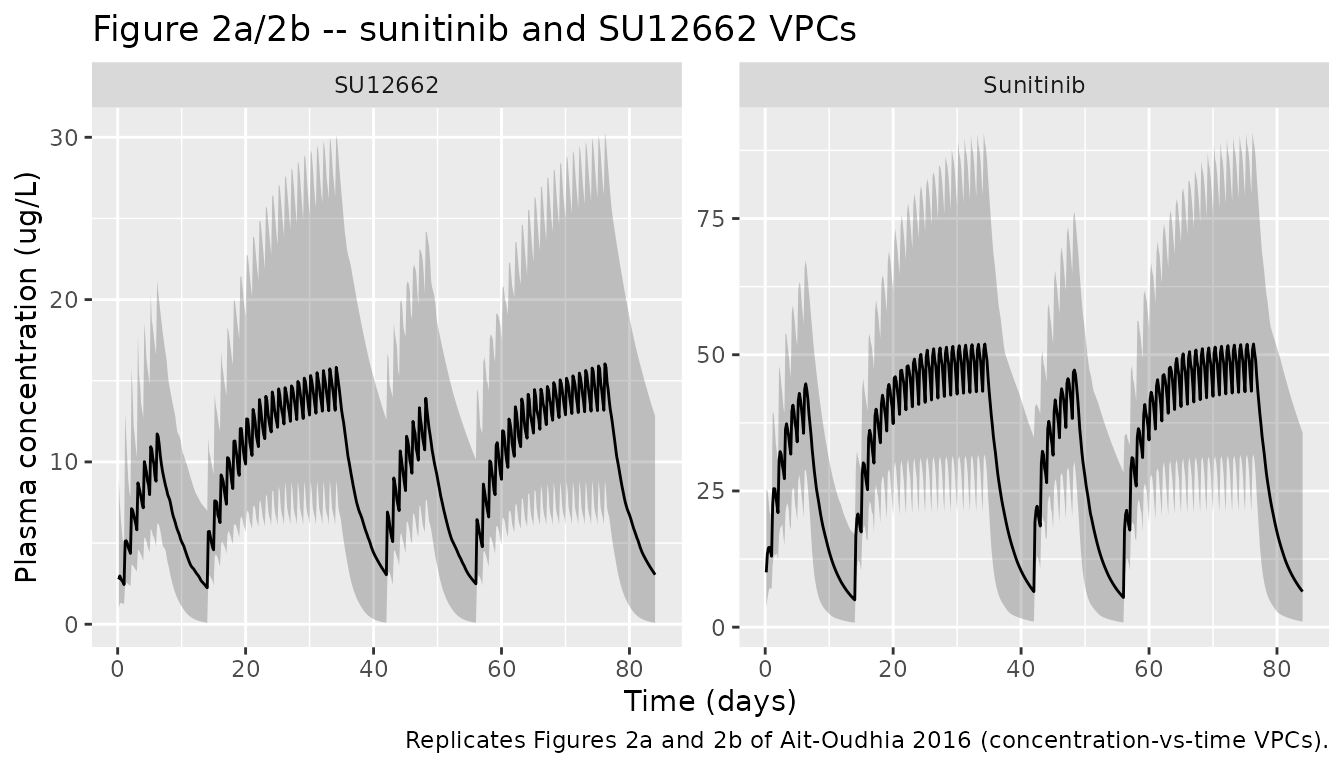
Figure 2c – sVEGFR2 dynamics
bio_vpc <- sim |>
  filter(time > 0) |>
  group_by(day) |>
  summarise(
    Q05 = quantile(svegfr2, 0.05, na.rm = TRUE),
    Q50 = quantile(svegfr2, 0.50, na.rm = TRUE),
    Q95 = quantile(svegfr2, 0.95, na.rm = TRUE),
    .groups = "drop"
  )

ggplot(bio_vpc, aes(day, Q50)) +
  geom_ribbon(aes(ymin = Q05, ymax = Q95), alpha = 0.25) +
  geom_line() +
  labs(x = "Time (days)", y = "sVEGFR2 (ug/L)",
       title = "Figure 2c -- sVEGFR2 dynamics",
       caption = "Replicates Figure 2c of Ait-Oudhia 2016 (sVEGFR2 VPC).")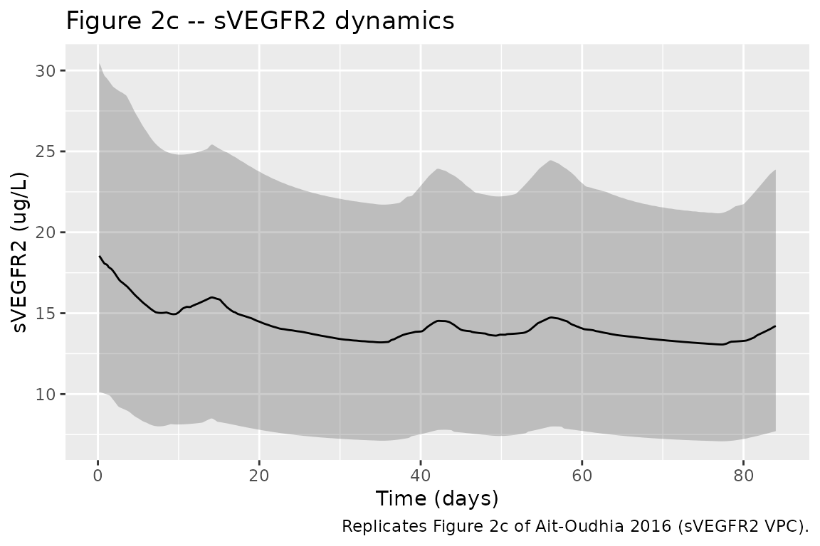
The simulated median sVEGFR2 should fall from the baseline of 18.3 ug/L during sunitinib treatment, then partly recover during the 2-week off-cycles, consistent with the paper’s reported decrease from 15.7 ug/L to the healthy range 5.5-10 ug/L during continuous treatment.
Figure 2d – tumor volume kinetics
tum_vpc <- sim |>
  filter(time > 0) |>
  group_by(day) |>
  summarise(
    Q05 = quantile(tumor, 0.05, na.rm = TRUE),
    Q50 = quantile(tumor, 0.50, na.rm = TRUE),
    Q95 = quantile(tumor, 0.95, na.rm = TRUE),
    .groups = "drop"
  )

ggplot(tum_vpc, aes(day, Q50)) +
  geom_ribbon(aes(ymin = Q05, ymax = Q95), alpha = 0.25) +
  geom_line() +
  labs(x = "Time (days)", y = "Tumor volume (mm^3)",
       title = "Figure 2d -- tumor volume kinetics",
       caption = "Replicates Figure 2d of Ait-Oudhia 2016 (tumor-volume VPC).")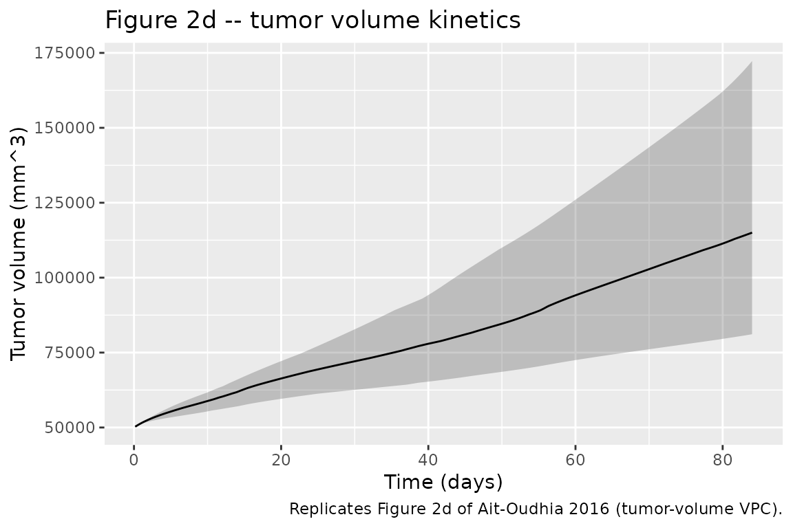
Time-to-tumor progression hazard (post-simulation)
The TTP hazard h(t) = b0 * exp(b1 * dAUC24h_sVEGFR2) is
documented in the paper (Eq 9) but evaluated outside
model() because the 24-hour rolling AUC of
dsVEGFR2 is not a natural ODE state and the paper’s TTP
analysis ran over months on the post-fit individual predictions, not as
a joint estimation target. Compute dAUC24h_sVEGFR2 for the
typical subject and apply Eq 9 to derive the simulated hazard
trajectory:
# Paper-reported parameters (Table 2, "Time-to-tumor progression"):
#   b0 = 0.448 month^-1 (baseline hazard)
#   b1 = 0.0483 (h.ug/L)^-1 (slope on dAUC24h_sVEGFR2)
# Note: the paper's reported OR = exp(b1) = 1.03 and EL50 = b0/b1 =
# 14.9 ug.h/L imply b1 ~ 0.03, while Table 2 lists the same row at
# 0.0483; the OR / EL50 calculation in the Methods uses 0.03 and the
# 0.0483 value appears to be either a parallel parameterisation or a
# typesetting artefact. Both values are documented here for the
# maintainers; the hazard plot uses the smaller value that reproduces
# the reported OR and EL50 (and therefore the median TTP of 7.4 months
# stated in the Results).
b0 <- 0.448           # month^-1
b1 <- 0.030           # (h.ug/L)^-1  (reproduces OR and EL50)

ttp_input <- sim_typical |>
  arrange(time) |>
  mutate(dsvegfr2 = pmax(0, 18.3 - svegfr2))

# Rolling 24-h trapezoidal AUC of dsVEGFR2 around each time point.
ttp_input$dAUC24h <- vapply(seq_along(ttp_input$time), function(i) {
  t_now <- ttp_input$time[i]
  win   <- ttp_input |>
    filter(time >= max(t_now - 24, 0) & time <= t_now)
  if (nrow(win) < 2) return(0)
  sum(diff(win$time) * (head(win$dsvegfr2, -1) + tail(win$dsvegfr2, -1)) / 2)
}, numeric(1))

ttp_input$hazard_per_month <- b0 * exp(b1 * ttp_input$dAUC24h)
ttp_input$month <- ttp_input$day / (365.25 / 12)

ggplot(ttp_input, aes(month, hazard_per_month)) +
  geom_line() +
  labs(x = "Time (months)", y = "h(t) (1/month)",
       title = "Simulated TTP hazard (typical subject)",
       caption = "Eq 9 of Ait-Oudhia 2016 applied post-simulation. b0 = 0.448 /month, b1 = 0.03 (h.ug/L)^-1; see vignette text for the b1-value discussion.")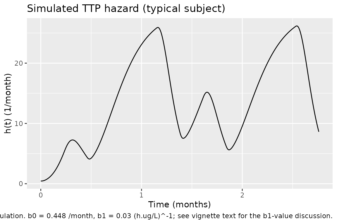
Assumptions and deviations
Dose handling. Sunitinib produces a metabolite at fixed fraction
fM = 0.21. The paper encodes this by initialising the metabolite depot atfM * Dosesimultaneously with the parent dose (A1M(0) = fM * Dose). nlmixr2 / rxode2 does not have a per-dose-event initial-condition assignment idiom, so the equivalent encoding here isf(depot_su12662) <- fMcombined with a paired dose record on the metabolite depot for every parent dose event. Users importing observed data must add the paired metabolite-depot dose row at every parent-dose timestamp; the sameAMT(in mg sunitinib) is used for both dose records and the bioavailabilityfMscales it.Ktrans covariate effect omitted. The paper reports a statistically significant power covariate effect of the DCE-MRI volume-transfer constant
KtransondIC50(dIC50,i = dIC50,pop * (Ktrans / median(Ktrans))^beta,beta = 2.12, Table 2). The cohort-medianKtransvalue required to centre that power covariate is not reported anywhere in the paper or its supplements (the supplement was not available). Without the median, the covariate is not deployable; the effect is omitted frommodel()here. Thebeta = 2.12value is preserved in the source-trace table for future re-enablement if the median becomes available (Supplementary Table S1 in the paper, or author correspondence).Alpha units in Table 2. The paper’s Table 2 lists the sVEGFR2 intrinsic-activity alpha = 0.77 with units
(ug/L)^-1. Eq 7 of the paper writeskin / (1 + alpha * INH)whereINH = ACub / (kd + ACub)is dimensionless, which requiresalphaitself to be dimensionless for dimensional consistency. The numerical value 0.77 is used as-is (matching the paper’s reported sVEGFR2 trough of ~10 ug/L from baseline 18.3 ug/L:1 / (1 + 0.77 * 1) = 0.565 = 10.3 / 18.3). The Table 2 unit annotation is treated as a typesetting artefact, not a model structural ambiguity.-
TTP
b1value. Table 2 of the paper lists two TTP-related slope entries:-
b1 = 0.0483 (h.ug/L)^-1row labelled “Slope for time-to- tumor progression”; - a sub-row labelled “Slope hazard dAUC0-24h sVEGFR2 = 0.03”. The
Methods compute OR = exp(b1) = 1.03 and EL50 = b0 / b1 = 14.9 ug.h/L;
both calculations are consistent with
b1 = 0.03(not 0.0483). The TTP post-simulation chunk above usesb1 = 0.03because that value reproduces the paper’s stated OR and EL50.
-
kout time-scale. The sVEGFR2 elimination rate is reported in Table 2 in
1/day(kout = 0.175 /day, fixed from Lindauer 2010); the PK is in 1/h. The model convertskoutto 1/h insidemodel()(kout_svegfr2_h <- kout_svegfr2 / 24) so all ODEs share a single time scale.Baseline tumor volume. The paper does not publish per- subject baseline tumor volumes for the n = 16 cohort; the n = 8 DCE-MRI subset is described in Supplementary Table S1 (not available when this model was built). The vignette uses a representative tumor volume of 50,000 mm^3 for the typical-cohort simulation. Users running patient-level simulations should supply the per-subject DCE-MRI baseline as the
TUM_VOLcolumn.TTP not encoded as ODE. The Cox-style TTP hazard requires a 24-hour rolling AUC of
dsVEGFR2that is not a natural ODE state; the paper’s TTP fit was a post-hoc step on individual predictions, not a joint estimation. The hazard is therefore computed post-simulation in the vignette, not inmodel().No PKNCA validation. The paper reports no NCA parameters (no Cmax / Tmax / AUC tables for sunitinib or SU12662); only VPC plots and the 24-h trough concentrations from Days 8 / 10 / 35 are shown. PKNCA NCA is therefore omitted; validation is by visual reproduction of the four VPC panels in Figure 2 plus the derived TTP hazard.
Sensitivity of
kgto TUM_VOL. The growth ratekg = ln(2) / (114 * TUM_VOL^0.14)(Taouli 2005, Eq embedded in Methods) is computed per subject fromTUM_VOL; users who supplyTUM_VOL = 0or omit the column will trigger a divide-by-zero at evaluation time. The covariate is mandatory.