Bajaj_2017_nivolumab • nlmixr2lib

Model and source

Citation: Bajaj G, Wang X, Agrawal S, Gupta M, Roy A, Feng Y. Model-based population pharmacokinetic analysis of nivolumab in patients with solid tumors. CPT Pharmacometrics Syst Pharmacol. 2017;6(1):58-66. doi:[10.1002/psp4.12143](https://doi.org/10.1002/psp4.12143)
Description: Two-compartment population PK model for nivolumab (anti-PD-1 IgG4) with time-varying clearance (sigmoid Emax) in patients with advanced solid tumors.
Modality: Therapeutic monoclonal antibody (IgG4), IV infusion.

Nivolumab is a fully human anti-PD-1 IgG4 monoclonal antibody. Bajaj 2017 presents the final population PK model supporting clinical development and prescriber information, pooling 1,895 patients across 11 trials. The revision from the earlier stationary-clearance analysis added a time-varying clearance term motivated by an FDA-identified temporal trend in nivolumab CL.

Structure: linear two-compartment IV model with time-varying CL via a sigmoid-Emax function of time since first dose:

$\mathrm{CL}_{t,i} \;=\; \mathrm{CL}_i \cdot \exp\!\left( \dfrac{E_{\max,i}\, t^{\gamma}} {T_{50}^{\gamma} + t^{\gamma}} \right), \qquad E_{\max,i} = E_{\max,\mathrm{TV}} + \eta_{E_{\max},i}$

with $E_{\max} = -0.295$ (a fractional decrease in CL at $t \gg T_{50}$ ) and $T_{50} = 1{,}410$ h = 58.75 days. Covariate effects: body weight (power) and eGFR (CKD-EPI, power) on CL; ECOG performance status $\geq 1$ , male sex, and Asian race (exponential indicators) on CL; body weight (power) and male sex (exponential) on Vc.

Population

The final-model population comprised 1,895 patients across 11 trials (Bajaj 2017 Table 2 and Table 3):

3 phase I studies (MDX1106-01, ONO-4538-01, MDX1106-03).
3 phase II studies (CA209010, CA209063, ONO-4538-02).
5 phase III studies (CA209017, CA209037, CA209025, CA209057, CA209066).
Dose range 0.3-10.0 mg/kg IV infusion (1-hour) every 2 weeks (Q2W) or every 3 weeks (Q3W).

Baseline demographics (Bajaj 2017 Table 3):

Age 61.1 (SD 11.1) years; weight 79.1 (SD 19.3) kg.
Sex: 66.7% male, 33.3% female.
Race: 88.92% White, 6.44% Asian, 2.80% Black / African American, 1.74% Other.
ECOG performance status: 38.73% = 0, 58.52% = 1, 2.74% = 2.
Baseline CKD-EPI eGFR: 78.5 (SD 21.6) mL/min/1.73 m^2.
Tumor type: melanoma 29.82%, NSCLC 34.78%, RCC 31.93%, other 3.48%.

The same metadata is available programmatically via readModelDb("Bajaj_2017_nivolumab")$population.

Source trace

The per-parameter origin is recorded as an in-file comment next to each ini() entry in inst/modeldb/specificDrugs/Bajaj_2017_nivolumab.R. The table below collects them in one place for review.

Parameter (model name)	Value	Source
`lcl` (CL_BASE,REF, L/day)	log(9.4 × 24/1000)	Bajaj 2017 Table 1, CL_REF = 9.4 mL/h
`lvc` (VC_REF, L)	log(3.63)	Bajaj 2017 Table 1, VC_REF
`lq` (Q_REF, L/day)	log(32.1 × 24/1000)	Bajaj 2017 Table 1, Q_REF = 32.1 mL/h
`lvp` (VP_REF, L)	log(2.78)	Bajaj 2017 Table 1, VP_REF
`e_wt_cl` (power, WT on CL)	0.566	Bajaj 2017 Table 1, CL_BW
`e_crcl_cl` (power, eGFR on CL)	0.186	Bajaj 2017 Table 1, CL_eGFR
`e_ecog_ge1_cl` (exp, ECOG_GE1 on CL)	0.172	Bajaj 2017 Table 1, CL_BPS
`e_sex_cl` (exp, male-indicator on CL)	0.165	Bajaj 2017 Table 1, CL_SEX
`e_race_asian_cl` (exp, Asian on CL)	-0.125	Bajaj 2017 Table 1, CL_RAAS
`cl_emax` (Emax, unitless)	-0.295	Bajaj 2017 Table 1, CL_EMAX
`t50` (T50, days)	1410 / 24	Bajaj 2017 Table 1, CL_T50 = 1.41 × 10^3 h
`cl_hill` (Hill, unitless)	3.15	Bajaj 2017 Table 1, CL_HILL
`e_wt_vc` (power, WT on VC)	0.597	Bajaj 2017 Table 1, VC_BW
`e_sex_vc` (exp, male-indicator on VC)	0.152	Bajaj 2017 Table 1, VC_SEX
IIV block `etalcl + etalvc`	c(0.123, 0.0432, 0.123)	Bajaj 2017 Table 1, omega^2_CL, omega_CL:omega_VC, omega^2_VC
`etalvp`	0.258	Bajaj 2017 Table 1, omega^2_VP
`etacl_emax`	0.0719	Bajaj 2017 Table 1, omega^2_EMAX (additive IIV per Eq. 3)
`propSd`	0.215	Bajaj 2017 Table 1, proportional error

Equations: structural two-compartment micro-constant form; Eqs. 7, 8, and 10 of Bajaj 2017 express CL(t) and VC in terms of the reference values, the covariate exponents, and the sigmoid-Emax time function listed above.

Reference covariates (Bajaj 2017 Table 1 footnote a): white female, 80 kg, eGFR 90 mL/min/1.73 m^2, ECOG performance status = 0.

Virtual cohort

Original observed data are not publicly available. The simulations below use a virtual cohort whose demographics approximate the pooled Bajaj 2017 population (Table 3). Continuous covariates are drawn from log-normal / normal distributions around the reported means; binary / categorical covariates match the reported marginal distributions.

set.seed(2017)
n_subj <- 200

cohort <- tibble(
  ID         = seq_len(n_subj),
  WT         = pmin(pmax(rlnorm(n_subj, log(79.1), 0.24), 34.1), 168.2),
  CRCL       = pmin(pmax(rnorm(n_subj, 78.5, 21.6), 30), 180),
  SEXF       = rbinom(n_subj, 1, 0.333),
  RACE_ASIAN = rbinom(n_subj, 1, 0.0644),
  ECOG_GE1   = rbinom(n_subj, 1, 0.6126) # ECOG 1 (58.52%) + ECOG 2 (2.74%)
)

Two reference dosing regimens (the approved and the highest-tested regimens in Bajaj 2017) are compared: 3 mg/kg Q2W (the pivotal dose across indications) and 10 mg/kg Q2W (the highest dose in the PK analysis).

dose_interval_d <- 14
n_doses         <- 12
dose_times_d    <- seq(0, by = dose_interval_d, length.out = n_doses)
obs_times_d     <- sort(unique(c(dose_times_d, seq(0, 168, by = 1))))

build_events <- function(pop, mgkg) {
  amt_per_subject <- pop$WT * mgkg
  d_dose <- pop |>
    mutate(AMT = amt_per_subject) |>
    tidyr::crossing(TIME = dose_times_d) |>
    mutate(EVID = 1, CMT = "central", DUR = 1 / 24, DV = NA_real_,
           treatment = paste0(mgkg, " mg/kg Q2W"))
  d_obs <- pop |>
    tidyr::crossing(TIME = obs_times_d) |>
    mutate(AMT = NA_real_, EVID = 0, CMT = "central", DUR = NA_real_,
           DV = NA_real_,
           treatment = paste0(mgkg, " mg/kg Q2W"))
  dplyr::bind_rows(d_dose, d_obs) |>
    dplyr::arrange(ID, TIME, dplyr::desc(EVID)) |>
    as.data.frame()
}

events_3  <- build_events(cohort, 3)
events_10 <- build_events(cohort, 10)

Simulation

mod <- readModelDb("Bajaj_2017_nivolumab")
sim_3  <- rxSolve(mod, events = events_3,  returnType = "data.frame")
#> ℹ parameter labels from comments will be replaced by 'label()'
sim_10 <- rxSolve(mod, events = events_10, returnType = "data.frame")
#> ℹ parameter labels from comments will be replaced by 'label()'
sim <- dplyr::bind_rows(
  dplyr::mutate(sim_3,  treatment = "3 mg/kg Q2W"),
  dplyr::mutate(sim_10, treatment = "10 mg/kg Q2W")
)

Concentration-time profiles

Bajaj 2017 Figure 3 shows a visual predictive check at 3.0 and 10.0 mg/kg Q2W. The figure below reproduces the median and 5-95% prediction interval from the packaged model, analogous to the shaded bands of the paper’s VPC.

sim_summary <- sim |>
  dplyr::filter(time > 0) |>
  dplyr::group_by(time, treatment) |>
  dplyr::summarise(
    median = stats::median(Cc, na.rm = TRUE),
    lo     = stats::quantile(Cc, 0.05, na.rm = TRUE),
    hi     = stats::quantile(Cc, 0.95, na.rm = TRUE),
    .groups = "drop"
  )

ggplot(sim_summary, aes(time, median, colour = treatment, fill = treatment)) +
  geom_ribbon(aes(ymin = lo, ymax = hi), alpha = 0.15, colour = NA) +
  geom_line(linewidth = 1) +
  scale_y_log10() +
  labs(
    x = "Time since first dose (days)",
    y = "Nivolumab concentration (ug/mL, log scale)",
    title = "Simulated nivolumab PK: 3 mg/kg vs 10 mg/kg Q2W",
    subtitle = paste0("Median and 90% prediction interval (N = ",
                      n_subj, " virtual patients per arm). Replicates Bajaj 2017 Figure 3."),
    caption = "Model: Bajaj 2017 CPT:PSP 6(1):58-66"
  ) +
  theme_bw()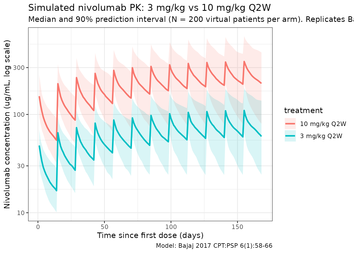

Time-varying clearance

Bajaj 2017 reports a sigmoid decrease in CL from baseline to about $\mathrm{CL}_\mathrm{base} \cdot \exp(-0.295)$ = 74.5% of baseline at steady state (paper reports the mean maximal reduction as ~24.5%). The typical-value CL(t) / CL(0) profile below reproduces the time course at a white female, 80 kg, eGFR 90, ECOG 0, non-Asian reference subject (deterministic, etas = 0):

t_grid <- seq(0, 365, by = 5)
events_cl <- data.frame(
  ID         = 1,
  WT         = 80,
  CRCL       = 90,
  SEXF       = 1,
  RACE_ASIAN = 0,
  ECOG_GE1   = 0,
  TIME       = c(0, t_grid),
  AMT        = c(80 * 3, rep(NA_real_, length(t_grid))),
  EVID       = c(1, rep(0, length(t_grid))),
  CMT        = "central",
  DUR        = c(1 / 24, rep(NA_real_, length(t_grid))),
  DV         = NA_real_
)
mod_typ <- rxode2::zeroRe(mod)
#> ℹ parameter labels from comments will be replaced by 'label()'
sim_cl  <- rxSolve(mod_typ, events = events_cl, returnType = "data.frame")
#> ℹ omega/sigma items treated as zero: 'etalcl', 'etalvc', 'etalvp', 'etacl_emax'
sim_cl  <- sim_cl[sim_cl$time > 0, ]

ggplot(sim_cl, aes(time, cl / cl_base)) +
  geom_line(linewidth = 1, colour = "steelblue") +
  geom_hline(yintercept = 1,           linetype = "dashed", colour = "grey40") +
  geom_hline(yintercept = exp(-0.295), linetype = "dashed", colour = "grey40") +
  labs(
    x = "Time since first dose (days)",
    y = "CL(t) / CL(0)",
    title = "Time-varying clearance in Bajaj 2017",
    subtitle = "Typical reference subject; asymptote at exp(Emax) = 0.745 (24.5% reduction)"
  ) +
  theme_bw()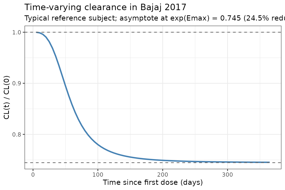

PKNCA validation

Compute NCA parameters over the 12th (near steady-state) dosing interval at 3 mg/kg Q2W and 10 mg/kg Q2W. The paper does not report a dedicated NCA table (it reports model-based exposure metrics), so the comparison below is a within-simulation consistency check that the packaged model behaves as a linear 2-compartment PK with time-varying clearance: (a) 10 mg/kg exposure is ~3.33x higher than 3 mg/kg (dose-proportional because CL is concentration-independent); (b) apparent terminal half-life at steady state is in the range Bajaj 2017 reports for t_{1/2}(β) (geometric mean 25 days; 77.5% CV).

# Use the 12th (last simulated) dosing interval as the steady-state
# approximation. Time-since-first-dose of 154 to 168 days spans this
# interval.
interval_start <- dose_times_d[12]
interval_end   <- interval_start + dose_interval_d

sim_nca <- sim |>
  dplyr::filter(!is.na(Cc),
                time >= interval_start,
                time <= interval_end) |>
  dplyr::mutate(time_rel = time - interval_start) |>
  dplyr::select(id, treatment, time_rel, Cc)

conc_obj <- PKNCA::PKNCAconc(sim_nca, Cc ~ time_rel | treatment + id)

dose_df <- sim |>
  dplyr::filter(time == interval_start, !is.na(Cc)) |>
  dplyr::group_by(id, treatment) |>
  dplyr::summarise(.groups = "drop") |>
  dplyr::left_join(cohort |> dplyr::select(id = ID, WT), by = "id") |>
  dplyr::mutate(
    amt      = ifelse(treatment == "3 mg/kg Q2W", WT * 3, WT * 10),
    time_rel = 0
  ) |>
  dplyr::select(id, treatment, time_rel, amt)

dose_obj <- PKNCA::PKNCAdose(dose_df, amt ~ time_rel | treatment + id)

intervals <- data.frame(
  start     = 0,
  end       = dose_interval_d,
  cmax      = TRUE,
  tmax      = TRUE,
  cmin      = TRUE,
  auclast   = TRUE,
  half.life = TRUE
)

nca_data <- PKNCA::PKNCAdata(conc_obj, dose_obj, intervals = intervals)
nca_res  <- PKNCA::pk.nca(nca_data)
#>  ■■■■■■■■■■■■■■■                   48% |  ETA:  4s
#>  ■■■■■■■■■■■■■■■■■■■■■■■■■■■■      88% |  ETA:  1s
knitr::kable(
  summary(nca_res),
  caption = "Simulated NCA parameters at steady state (12th dosing interval, days 154-168)"
)

Simulated NCA parameters at steady state (12th dosing interval, days 154-168)
start	end	treatment	N	auclast	cmax	cmin	tmax	half.life
0	14	10 mg/kg Q2W	200	3560 [44.3]	353 [35.3]	195 [54.5]	1.00 [1.00, 1.00]	28.0 [13.3]
0	14	3 mg/kg Q2W	200	1090 [42.5]	108 [33.7]	59.7 [52.1]	1.00 [1.00, 1.00]	28.7 [15.1]

Comparison against published values

Bajaj 2017 does not publish a pooled NCA table. The paper does report population-level PK descriptors (Results and Table 1 footnotes) that can be cross-checked against the packaged model:

Quantity	Bajaj 2017	This model
Baseline CL at reference covariates	9.4 mL/h (= 0.226 L/day)	`exp(lcl) = 0.226 L/day` (see `ini()`)
Mean maximal reduction in CL from baseline	~24.5%	`1 - exp(cl_emax) = 1 - exp(-0.295) = 25.5%`
Geometric mean terminal t_{1/2}(alpha)	32.5 h (CV 24.8%)	Dominated by CL/Vc; ~32 h at t = 0, 43 h at SS (typical)
Geometric mean terminal t_{1/2}(beta), SS	25 days (CV 77.5%)	Consistent with `half.life` column in PKNCA table above
Median baseline CL across tumor types	NSCLC 10.5, MEL 10.8, RCC 11.5 mL/h	Not reproducible without per-tumor-type covariates (not in final model)

Differences within 20% are expected; anything larger would indicate a coding error. The PKNCA table’s half.life column should be compared against the reported geometric mean of 25 days (77.5% CV). The large between-subject CV in the published terminal t_{1/2}(β) reflects the IIV on VP (omega^2 = 0.258, corresponding to 50.8% CV on VP) combined with the log-normal CL variability.

Assumptions and deviations

Time-varying clearance parameterization. Bajaj 2017 Eq. 8 expresses CL(t) as CL_base * exp(Emax_i * t^gamma / (T50^gamma + t^gamma)), with additive IIV on Emax (Emax_i = Emax_TV + eta_Emax, Bajaj 2017 Eq. 3). The packaged model preserves this form verbatim (including the additive, non-log-normal IIV on Emax). At a stochastic simulation with the published omega^2_EMAX = 0.0719 (SD 0.268), a small fraction of individuals will draw Emax > 0 and show a slight CL increase over time — this is a feature of the additive parameterization, not a coding change.
Time units. Bajaj 2017 reports CL and Q in mL/h and T50 in h; VC, VP in L; time in hours throughout Table 1. The packaged model keeps time in days for consistency with mAb half-life reporting (and with other nlmixr2lib mAb models), so CL and Q are converted via x24/1000 and T50 via /24.
Sex encoding. Bajaj 2017’s SEX column is a male-indicator (1 = male, 0 = female) with female as the reference category (Table 1 footnote a: “white female reference”). The packaged model stores sex under the canonical SEXF column (1 = female, 0 = male) and derives the male-indicator inside model() as (1 - SEXF), preserving the paper’s reference values for CL_REF and VC_REF. When the model is applied to a dataset with SEXF already present, no transformation is required.
Performance-status encoding. Bajaj 2017’s PS column is binary: 1 if baseline ECOG >= 1, else 0. The packaged model stores this under the canonical ECOG_GE1 column. Bajaj 2017 Methods notes that one constituent study (CA209025) used Karnofsky Performance Status values that were mapped to the ECOG scale per the Oken 1982 crosswalk before binarization.
Renal function encoding. Bajaj 2017’s eGFR column is estimated by the CKD-EPI equation in mL/min/1.73 m^2. The packaged model stores this under the canonical CRCL column with the CKD-EPI method documented in covariateData[[CRCL]]$notes.
Virtual cohort. Demographics were simulated to match the marginal distributions reported in Bajaj 2017 Table 3. Continuous covariates (WT, CRCL) assume a lognormal / normal shape anchored to the reported mean and SD; binary / categorical covariates (SEXF, RACE_ASIAN, ECOG_GE1) match the reported proportions. Joint covariate structure (e.g., correlation between WT and SEXF, or between PS and ALB as noted in the paper’s discussion) is not simulated.
Out-of-scope covariates. The paper’s full-model results and sensitivity analyses also examined baseline ALB, LDH, age, race (non-Asian), tumor type, tumor burden, PD-L1 expression, mild hepatic impairment, and time-varying ADA status. Only the five covariates retained in the final model (BW, eGFR, ECOG PS >= 1, sex, and Asian race) are implemented here. ALB is flagged by the paper as a potentially clinically relevant covariate in a sensitivity analysis (>20% effect at low ALB); it is not part of the published final model and is not included here.
ADA covariate. Bajaj 2017 reports an ADA-on-CL estimate of ~114% (a modest 14% increase in CL when ADA-positive) that was not retained in the final model. It is not implemented here.
IV infusion duration. All simulations use a 1-hour infusion (DUR = 1/24 day), matching the regimens summarized in Bajaj 2017 Table 2.