Cephalexin (Haynes 2025)
Source:vignettes/articles/Haynes_2025_cephalexin.Rmd
Haynes_2025_cephalexin.Rmd
mod <- readModelDb("Haynes_2025_cephalexin")
ui <- rxode2::rxode(mod)
Model and source
- Citation: Haynes AS, Wei Z, Scheetz MH, Gonzalez D, Messacar K, Tang Girdwood S, Peloquin CA, Fish DN, Anderson P. Oral Cephalexin Population Pharmacokinetics and Target Attainment Analysis in Infants 7-60 Days Old. J Pediatric Infect Dis Soc. 2025;14(10):piaf088. doi:10.1093/jpids/piaf088
- Description: One-compartment oral population PK model for cephalexin in neonates and young infants 7-60 days old (Haynes 2025; NCT04916951, Children’s Hospital Colorado). First-order absorption with an absorption lag time and linear elimination. Apparent clearance (CL/F) and apparent volume of distribution (Vd/F) are scaled to body weight with exponents fixed to 0.75 and 1.0 respectively (reference 70 kg), with an estimated power effect of postmenstrual age on CL/F (reference 41.06 weeks) and of postnatal age on the absorption rate constant (reference 29.14 days). Inter-individual variability is estimated on lag time, absorption rate constant and CL/F but not on Vd/F; residual error is combined additive plus proportional.
- Article: https://doi.org/10.1093/jpids/piaf088
- Trial registration: NCT04916951
Cephalexin is an oral first-generation cephalosporin. Transitioning young infants from intravenous to oral antibiotics is uncommon because there are almost no pharmacokinetic data to support oral dosing in the first two months of life, when gastrointestinal absorption and renal function are both maturing rapidly. Haynes 2025 fitted a population PK model to prospectively collected cephalexin concentrations in hospitalized infants and then used it to identify oral regimens that achieve free-drug time above the MIC (fT>MIC) targets for common neonatal pathogens.
The final model is a one-compartment model with first-order
absorption, an absorption lag time, and linear elimination. Because all
doses were enteral, the disposition parameters are apparent
(CL/F, Vd/F) and no separate bioavailability
term is identifiable.
Population
Thirty-three hospitalized infants contributed 144 cephalexin plasma concentrations after data cleaning (Haynes 2025 Table 1, with Tables S1-S2). Median postnatal age was 31.16 days (range 9.49-56.54) and median gestational age at birth was 37 2/7 weeks (range 29 3/7 to 40 6/7), so the cohort spans late-preterm through term infants. Median weight was 3.36 kg (range 2.20-5.39) and 30% were female. Race was reported as White in 70%, Asian in 9% and unknown or not reported in 21%; 30% were Hispanic. Nine infants were enrolled while receiving enteral cephalexin as standard of care and 24 received a single 25 mg/kg enteral research dose while on IV antibiotics. Doses ranged from 12.0 to 29.5 mg/kg (median 24.7); one infant received 12.0 mg/kg and all others 22.5-29.5 mg/kg. Most doses were given through a gastric tube (20 of 33) rather than by mouth (10 of 33) or a post-pyloric tube (3 of 33). Median eGFR was 68.8 mL/min/1.73 m^2 (range 37.8-126.1), available within 48 h of dosing for 25 of 33 infants. Sampling was sparse: 3-5 samples per infant across 1-5 dosing intervals.
The same information is available programmatically via the model’s
population metadata
(readModelDb("Haynes_2025_cephalexin")()$population).
str(ui$population)
#> List of 17
#>  $ species       : chr "human"
#>  $ n_subjects    : int 33
#>  $ n_studies     : int 1
#>  $ n_observations: int 144
#>  $ age_range     : chr "9.49-56.54 days postnatal"
#>  $ age_median    : chr "31.16 days postnatal"
#>  $ ga_range      : chr "29 3/7 to 40 6/7 weeks gestational age at birth"
#>  $ ga_median     : chr "37 2/7 weeks gestational age at birth"
#>  $ weight_range  : chr "2.20-5.39 kg"
#>  $ weight_median : chr "3.36 kg"
#>  $ sex_female_pct: num 30
#>  $ race_ethnicity: Named num [1:8] 70 0 9 0 21 30 58 12
#>   ..- attr(*, "names")= chr [1:8] "White" "Black" "Asian" "Native Hawaiian/Other Pacific Islander" ...
#>  $ disease_state : chr "Hospitalized neonates and young infants receiving antibiotics, enrolled either while receiving enteral cephalex"| __truncated__
#>  $ renal_function: chr "eGFR median 68.8 mL/min/1.73 m^2 (range 37.8-126.1); available within 48 h of dosing for 25 of 33 subjects"
#>  $ dose_range    : chr "12.0-29.5 mg/kg per dose as an oral suspension (median 24.7 mg/kg); one subject received 12.0 mg/kg and all oth"| __truncated__
#>  $ regions       : chr "United States (single center: Children's Hospital Colorado, Aurora, CO)"
#>  $ notes         : chr "Baseline demographics, dosing, sampling and laboratory availability are in Haynes 2025 Table 1 (with Tables S1-"| __truncated__
Source trace
The per-parameter origin is recorded as an in-file comment next to
each ini() entry in
inst/modeldb/specificDrugs/Haynes_2025_cephalexin.R. The
table below collects them in one place for review. All values come from
the peer-reviewed paper; see Assumptions and deviations for why
the earlier conference abstract of the same work is not
the source.
| Equation / parameter | Value | Source location |
|---|---|---|
| One-compartment, first-order absorption, lag time, linear elimination | structure | Results, “Final Model” |
Tlag_i = Tlag_pop * exp(eta_Tlag) |
equation | Results, “Final Model”, eq. 1 |
Ka_i = Ka_pop * (PNA / 29.14)^beta_PNA * exp(eta_Ka) |
equation | Results, “Final Model”, eq. 2 |
Vd_i/F = Vd_pop/F * (WT / 70)^1 |
equation | Results, “Final Model”, eq. 3 |
CL_i/F = CL_pop/F * (WT / 70)^0.75 * (PMA / 41.06)^beta_PMA * exp(eta_CL) |
equation | Results, “Final Model”, eq. 4 |
ltlag (Tlag) |
0.61 h (RSE 21.0%, CI 0.41-0.91) | Table 2, “Lag time (Tlag, h)” |
lka (Ka) |
1.32 1/h (RSE 21.2%, CI 0.88-1.97) | Table 2, “Absorption rate constant (Ka, 1/h)” |
lvc (Vd/F) |
30.63 L/70 kg (RSE 5.64%, CI 27.43-34.20) | Table 2, “Apparent volume of distribution (Vd/F, L/70kg)” |
lcl (CL/F) |
6.33 L/h/70 kg (RSE 4.49%, CI 5.80-6.91) | Table 2, “Apparent clearance (Cl/F, L/h/70kg)” |
e_pna_ka |
0.92 (RSE 33.0%, CI 0.32-1.52) | Table 2, “beta PNA_Ka” |
e_page_cl |
2.92 (RSE 19.7%, CI 1.79-4.05) | Table 2, “beta PMA_CL” |
e_wt_cl |
0.75, fixed | Table 2 “beta WT_CL” (no RSE); Results “exponent fixed to 0.75” |
e_wt_vc |
1.00, fixed | Table 2 “beta WT_V” (no RSE); Results “linear scaling … exponent fixed to 1.0” |
etaltlag |
SD 0.74 -> var 0.5476 (RSE 20.9%, CI 0.50-1.10) | Table 2, “IIV for Tlag” |
etalka |
SD 0.63 -> var 0.3969 (RSE 24.2%, CI 0.40-0.99) | Table 2, “IIV for Ka” |
etalcl |
SD 0.20 -> var 0.04 (RSE 18.5%, CI 0.14-0.29) | Table 2, “IIV for Cl/F” |
addSd |
0.26 mg/L (RSE 41.8%, CI 0.12-0.54) | Table 2, “constant (a, mg/L)” |
propSd |
0.22 (RSE 13.0%, CI 0.17-0.28) | Table 2, “proportional (b)” |
| PNA reference | 29.14 days | Results, “Final Model”, eq. 2 denominator |
| PMA reference | 41.06 weeks | Results, “Final Model”, eq. 4 denominator |
| Weight reference | 70 kg | Results, “Final Model”, eqs. 3-4 denominators |
| Protein binding (simulations only) | 10% | Methods, “Dosing Simulations” |
Omega scale: SD, not variance
Haynes 2025 Table 2 reports the random effects under the heading
Standard Deviation of the Random Effects, with a
Value column next to a C.V.(%) column. Reading
Value as a log-scale SD reproduces the printed CVs through
CV = sqrt(exp(omega^2) - 1), which confirms the scale and
rules out reading those numbers as variances.
omega_sd <- c(0.74, 0.63, 0.20)
printed_cv <- c(85.35, 70.19, 20.66)
omega_check <- data.frame(
  Parameter = c("Tlag", "Ka", "Cl/F"),
  `Table 2 SD` = omega_sd,
  `CV if SD (%)` = round(100 * sqrt(exp(omega_sd^2) - 1), 2),
  `CV if variance (%)` = round(100 * sqrt(exp(omega_sd) - 1), 2),
  `Table 2 CV (%)` = printed_cv,
  check.names = FALSE
)
knitr::kable(omega_check, row.names = FALSE)| Parameter | Table 2 SD | CV if SD (%) | CV if variance (%) | Table 2 CV (%) |
|---|---|---|---|---|
| Tlag | 0.74 | 85.39 | 104.69 | 85.35 |
| Ka | 0.63 | 69.80 | 93.68 | 70.19 |
| Cl/F | 0.20 | 20.20 | 47.05 | 20.66 |
# The SD reading reproduces every printed CV to within rounding of the
# 2-decimal SD; the variance reading is off by tens of percent. Deterministic
# arithmetic, so the bound is tight.
stopifnot(all(abs(omega_check$`CV if SD (%)` - printed_cv) < 0.6))
stopifnot(all(abs(omega_check$`CV if variance (%)` - printed_cv) > 5))
Structural verification against the closed form
A one-compartment model with first-order absorption, an absorption
lag tlag and apparent volume vc has the
closed-form single-dose solution
and for . Solving the packaged ODE model and comparing it against this expression tests that the ODE structure, the lag placement and the covariate algebra were transcribed correctly.
This gate runs on a deterministic covariate grid with the random effects zeroed, so it involves no random draws and both sides use identical parameters. The residual difference is pure ODE-solver error, so a tight bound is the correct assertion here, unlike the cohort-level checks further down.
mod_typ <- rxode2::zeroRe(mod)

# Four deterministic covariate combinations spanning the observed cohort:
# a small late-preterm newborn through a large 8-week-old term infant.
grid_cov <- data.frame(
  id = 1:4,
  label = c(
    "2.0 kg, GA 31 wk, PNA 10 d", "3.36 kg, GA 37.3 wk, PNA 31 d",
    "4.5 kg, GA 39 wk, PNA 50 d", "5.4 kg, GA 40 wk, PNA 56 d"
  ),
  WT = c(2.00, 3.36, 4.50, 5.40),
  GA = c(31, 37 + 2 / 7, 39, 40),
  pna_days = c(10, 31, 50, 56),
  stringsAsFactors = FALSE
)
grid_cov <- grid_cov |>
  mutate(
    PNA = pna_days / 30.4375,  # canonical PNA is carried in months
    PAGE = GA + pna_days / 7,  # postmenstrual age in weeks
    dose_mg = 25 * WT          # 25 mg/kg, the study research dose
  )

# 12 h is ~7 elimination half-lives for this model. Going much further pushes
# the tail into solver noise, where a relative comparison is meaningless and
# PKNCA's terminal-slope fit can take log() of a negative value.
t_grid <- seq(0, 12, by = 0.05)

ev_typ <- bind_rows(
  grid_cov |> mutate(time = 0, amt = dose_mg, evid = 1L, cmt = "depot"),
  grid_cov |>
    tidyr::crossing(time = t_grid) |>
    mutate(amt = NA_real_, evid = 0L, cmt = "central")
) |>
  arrange(id, time, desc(evid)) |>
  select(id, time, amt, evid, cmt, WT, PNA, PAGE, dose_mg, label)

sim_typ <- rxode2::rxSolve(
  mod_typ, ev_typ,
  keep = c("WT", "PNA", "PAGE", "dose_mg", "label")
) |>
  as.data.frame() |>
  filter(!is.na(Cc))
#> ℹ omega/sigma items treated as zero: 'etaltlag', 'etalka', 'etalcl'
#> Warning: multi-subject simulation without without 'omega'

closed_form <- function(t, dose, ka, kel, vc, tlag) {
  te <- pmax(t - tlag, 0)
  ifelse(
    t < tlag, 0,
    (dose / vc) * (ka / (ka - kel)) * (exp(-kel * te) - exp(-ka * te))
  )
}

cf_chk <- sim_typ |>
  mutate(Cc_cf = closed_form(time, dose_mg, ka, kel, vc, tlag)) |>
  group_by(label) |>
  summarise(
    ka = first(ka), kel = first(kel), vc = first(vc), tlag = first(tlag),
    max_abs_diff = max(abs(Cc - Cc_cf)),
    max_rel_diff_pct = 100 * max(abs(Cc - Cc_cf) / pmax(Cc_cf, 1e-6)),
    .groups = "drop"
  )

knitr::kable(cf_chk, digits = c(0, 3, 4, 3, 3, 9, 6))| label | ka | kel | vc | tlag | max_abs_diff | max_rel_diff_pct |
|---|---|---|---|---|---|---|
| 2.0 kg, GA 31 wk, PNA 10 d | 0.493 | 0.2523 | 0.875 | 0.61 | 2.980e-07 | 2.0e-05 |
| 3.36 kg, GA 37.3 wk, PNA 31 d | 1.397 | 0.4624 | 1.470 | 0.61 | 2.511e-06 | 2.0e-05 |
| 4.5 kg, GA 39 wk, PNA 50 d | 2.169 | 0.5771 | 1.969 | 0.61 | 6.390e-06 | 3.5e-05 |
| 5.4 kg, GA 40 wk, PNA 56 d | 2.408 | 0.6187 | 2.363 | 0.61 | 6.715e-06 | 4.3e-05 |
# ka and kel must stay well separated for the closed form to be well
# conditioned; confirm that before trusting the comparison.
stopifnot(all(abs(cf_chk$ka - cf_chk$kel) / cf_chk$kel > 0.5))
# Deterministic solve vs its own closed form: solver error only.
stopifnot(max(cf_chk$max_abs_diff) < 1e-5)
stopifnot(max(cf_chk$max_rel_diff_pct) < 0.05)

# The lag must actually delay absorption: every pre-lag concentration is zero.
pre_lag <- sim_typ |> filter(time < tlag - 1e-9)
stopifnot(nrow(pre_lag) > 0, all(pre_lag$Cc == 0))
The pre-lag rows are asserted to exist as well as to be zero, so the check cannot pass by matching no rows.
Covariate model verification
The two estimated covariate effects are power functions. At the reference covariate values they must collapse to the reported typical parameters, and away from the reference they must move in the direction the paper describes: absorption faster with increasing postnatal age, and apparent clearance higher with increasing postmenstrual age.
# Event tables for reading back individual parameters MUST carry observation
# rows. Given only dose records, rxode2 invents its own observation grid and
# the covariate columns come back as NA for every subject but the first, so a
# multi-subject dose-only table silently evaluates one subject's covariates
# for the whole grid.
param_events <- function(d) {
  bind_rows(
    d |> mutate(time = 0, amt = 1, evid = 1L, cmt = "depot"),
    d |>
      tidyr::crossing(time = c(0, 1, 2)) |>
      mutate(amt = NA_real_, evid = 0L, cmt = "central")
  ) |>
    arrange(id, time, desc(evid)) |>
    select(id, time, amt, evid, cmt, dplyr::everything())
}

# A "reference" infant sitting exactly at the printed reference values, scaled
# to 70 kg so the allometric terms are 1 as well.
ref_ind <- param_events(
  data.frame(id = 1L, WT = 70, PNA = 29.14 / 30.4375, PAGE = 41.06)
)
ref_par <- rxode2::rxSolve(mod_typ, ref_ind) |> as.data.frame()
#> ℹ omega/sigma items treated as zero: 'etaltlag', 'etalka', 'etalcl'
stopifnot(nrow(ref_par) > 0, !is.na(ref_par$cl[1]))

ref_tab <- data.frame(
  Parameter = c("Tlag (h)", "Ka (1/h)", "Vd/F (L/70 kg)", "CL/F (L/h/70 kg)"),
  Model = c(ref_par$tlag[1], ref_par$ka[1], ref_par$vc[1], ref_par$cl[1]),
  `Table 2` = c(0.61, 1.32, 30.63, 6.33),
  check.names = FALSE
)
ref_tab$`Diff (%)` <- 100 * (ref_tab$Model - ref_tab$`Table 2`) / ref_tab$`Table 2`
knitr::kable(ref_tab, digits = 6)| Parameter | Model | Table 2 | Diff (%) |
|---|---|---|---|
| Tlag (h) | 0.61 | 0.61 | 0 |
| Ka (1/h) | 1.32 | 1.32 | 0 |
| Vd/F (L/70 kg) | 30.63 | 30.63 | 0 |
| CL/F (L/h/70 kg) | 6.33 | 6.33 | 0 |
# At the reference covariates the model must return the printed typicals
# exactly; only floating point separates them.
stopifnot(max(abs(ref_tab$`Diff (%)`)) < 1e-6)

# Maturation directions, evaluated deterministically over the covariate ranges.
mat <- expand.grid(pna_days = c(7, 14, 28, 42, 60), GA = c(32, 40)) |>
  mutate(
    id = dplyr::row_number(), WT = 3.36,
    PNA = pna_days / 30.4375, PAGE = GA + pna_days / 7
  ) |>
  param_events()
mat_par <- rxode2::rxSolve(mod_typ, mat, keep = c("pna_days", "GA")) |>
  as.data.frame() |>
  group_by(pna_days, GA) |>
  summarise(ka = first(ka), cl = first(cl), .groups = "drop") |>
  arrange(GA, pna_days)
#> ℹ omega/sigma items treated as zero: 'etaltlag', 'etalka', 'etalcl'
#> Warning: multi-subject simulation without without 'omega'
knitr::kable(mat_par, digits = 3)| pna_days | GA | ka | cl |
|---|---|---|---|
| 7 | 32 | 0.355 | 0.343 |
| 14 | 32 | 0.672 | 0.374 |
| 28 | 32 | 1.272 | 0.442 |
| 42 | 32 | 1.848 | 0.518 |
| 60 | 32 | 2.565 | 0.627 |
| 7 | 40 | 0.355 | 0.646 |
| 14 | 40 | 0.672 | 0.693 |
| 28 | 40 | 1.272 | 0.794 |
| 42 | 40 | 1.848 | 0.904 |
| 60 | 40 | 2.565 | 1.060 |
# Guard the grid shape and confirm the covariates actually arrived, so the
# monotonicity assertions below cannot pass on an NA-collapsed grid.
stopifnot(nrow(mat_par) == 10L, !anyNA(mat_par$ka), !anyNA(mat_par$cl))

# These effects are strong and computed deterministically, so a step-by-step
# monotonicity assertion is safe here (no cohort noise to flip a pair).
for (g in unique(mat_par$GA)) {
  sub <- mat_par |> filter(GA == g) |> arrange(pna_days)
  stopifnot(nrow(sub) == 5L)
  stopifnot(all(diff(sub$ka) > 0))  # ka rises with postnatal age
  stopifnot(all(diff(sub$cl) > 0))  # CL/F rises with postmenstrual age
}
# A term infant clears faster than a preterm infant of the same weight and
# postnatal age, because postmenstrual age is higher.
wide_mat <- mat_par |>
  tidyr::pivot_wider(names_from = GA, values_from = c(ka, cl))
stopifnot(nrow(wide_mat) == 5L)
stopifnot(all(wide_mat$cl_40 > wide_mat$cl_32))
# Gestational age enters ka nowhere, so ka must be identical across GA strata.
stopifnot(max(abs(wide_mat$ka_40 - wide_mat$ka_32)) < 1e-10)
Virtual cohort
The paper’s dosing simulations used a 20,000-subject virtual population generated in PK-Sim and stratified by gestational age (30-34 vs >= 35 weeks) and postnatal age (7-28 vs 29-60 days) into four groups. The underlying weight / GA / PNA distributions are in Figure S1, which is not in the accessible portion of the record, so the cohort below is reconstructed from a documented weight-for-age approximation rather than copied. It is sized at 200 infants per stratum, the per-arm cap for these vignettes.
n_per_arm <- 200L

arm_levels <- c(
  "GA <35 wk, PNA 7-28 d", "GA >=35 wk, PNA 7-28 d",
  "GA <35 wk, PNA 29-60 d", "GA >=35 wk, PNA 29-60 d"
)

# Approximate 50th-percentile birth weight by gestational age (kg), close to
# the Fenton / WHO reference curves. Interpolated linearly between knots.
bw_knots <- data.frame(
  GA = c(30, 32, 34, 36, 38, 40),
  BW = c(1.4, 1.8, 2.3, 2.8, 3.2, 3.5)
)
birth_weight <- function(ga) {
  stats::approx(bw_knots$GA, bw_knots$BW, xout = ga, rule = 2)$y
}

make_arm <- function(ga_lo, ga_hi, pna_lo, pna_hi, arm, seed) {
  # Seed each stochastic block separately so the cohort is reproducible and
  # each arm draws its own stream.
  set.seed(seed)
  ga <- stats::runif(n_per_arm, ga_lo, ga_hi)
  pna_days <- stats::runif(n_per_arm, pna_lo, pna_hi)
  # ~5% initial weight loss then ~25 g/day of postnatal gain from day 7,
  # with a 12% lognormal CV for between-infant spread.
  wt <- (birth_weight(ga) * 0.95 + 0.025 * (pna_days - 7)) *
    stats::rlnorm(n_per_arm, 0, 0.12)
  data.frame(
    arm = arm, GA = ga, pna_days = pna_days, WT = wt,
    PNA = pna_days / 30.4375, PAGE = ga + pna_days / 7,
    stringsAsFactors = FALSE
  )
}

cohort <- bind_rows(
  make_arm(30, 34.999, 7, 28, arm_levels[1], 20250001),
  make_arm(35, 40.999, 7, 28, arm_levels[2], 20250002),
  make_arm(30, 34.999, 29, 60, arm_levels[3], 20250003),
  make_arm(35, 40.999, 29, 60, arm_levels[4], 20250004)
) |>
  mutate(id = dplyr::row_number())

cohort |>
  mutate(arm = factor(arm, levels = arm_levels)) |>
  group_by(arm) |>
  summarise(
    n = n(),
    `GA (wk)` = sprintf("%.1f (%.1f-%.1f)", median(GA), min(GA), max(GA)),
    `PNA (d)` = sprintf("%.0f (%.0f-%.0f)", median(pna_days), min(pna_days), max(pna_days)),
    `PMA (wk)` = sprintf("%.1f (%.1f-%.1f)", median(PAGE), min(PAGE), max(PAGE)),
    `WT (kg)` = sprintf("%.2f (%.2f-%.2f)", median(WT), min(WT), max(WT)),
    .groups = "drop"
  ) |>
knitr::kable(caption = "Reconstructed virtual cohort, median (range).")| arm | n | GA (wk) | PNA (d) | PMA (wk) | WT (kg) |
|---|---|---|---|---|---|
| GA <35 wk, PNA 7-28 d | 200 | 32.9 (30.0-35.0) | 18 (7-28) | 35.3 (31.3-38.6) | 2.14 (1.28-3.44) |
| GA >=35 wk, PNA 7-28 d | 200 | 37.4 (35.0-41.0) | 18 (7-28) | 40.1 (36.5-44.3) | 3.18 (2.16-4.54) |
| GA <35 wk, PNA 29-60 d | 200 | 32.6 (30.0-35.0) | 45 (29-60) | 38.9 (34.6-42.7) | 2.73 (1.74-4.23) |
| GA >=35 wk, PNA 29-60 d | 200 | 38.0 (35.0-40.9) | 45 (29-60) | 44.5 (39.5-49.0) | 3.95 (2.49-5.55) |
The reconstructed weights bracket the study cohort’s observed 2.20-5.39 kg range, which is the only published check available on them.
Single-dose simulation
A single 25 mg/kg oral dose, matching the research dose given to 24 of the 33 study infants, simulated with full inter-individual variability.
rxode2::rxSetSeed(20250101)

sd_grid <- c(seq(0, 2, by = 0.05), seq(2.25, 6, by = 0.25), seq(6.5, 12, by = 0.5))

ev_sd <- bind_rows(
  cohort |> mutate(time = 0, amt = 25 * WT, evid = 1L, cmt = "depot"),
  cohort |>
    tidyr::crossing(time = sd_grid) |>
    mutate(amt = NA_real_, evid = 0L, cmt = "central")
) |>
  mutate(dose_mg = 25 * WT) |>
  arrange(id, time, desc(evid)) |>
  select(id, time, amt, evid, cmt, WT, PNA, PAGE, arm, dose_mg)

sim_sd <- rxode2::rxSolve(mod, ev_sd, keep = c("WT", "arm", "dose_mg")) |>
  as.data.frame()

# rxSolve drops the id column for a single subject; this cohort has many, but
# check rather than assume (and the observable must be finite everywhere).
stopifnot(!is.null(sim_sd$id))
stopifnot(all(is.finite(sim_sd$Cc[!is.na(sim_sd$Cc)])))
stopifnot(all(sim_sd$Cc[!is.na(sim_sd$Cc)] >= 0))
sim_sd |>
  filter(!is.na(Cc)) |>
  mutate(arm = factor(arm, levels = arm_levels)) |>
  group_by(arm, time) |>
  summarise(
    med = median(Cc), lo = quantile(Cc, 0.05), hi = quantile(Cc, 0.95),
    .groups = "drop"
  ) |>
  ggplot(aes(time, med, ymin = lo, ymax = hi, fill = arm, colour = arm)) +
  geom_ribbon(alpha = 0.2, colour = NA) +
  geom_line(linewidth = 0.7) +
  labs(
    x = "Time after dose (h)", y = "Cephalexin concentration (mg/L)",
    colour = NULL, fill = NULL
  ) +
  theme_bw() +
  theme(legend.position = "bottom")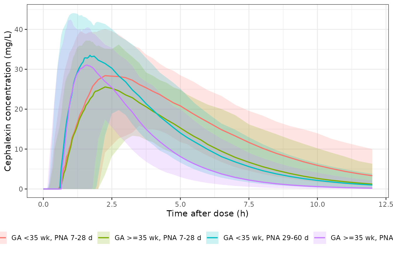
Simulated cephalexin plasma concentrations after a single 25 mg/kg oral dose, by gestational- and postnatal-age stratum. Line = median, band = 5th-95th percentile.
PKNCA validation
NCA is run with PKNCA on the simulated single-dose profiles, grouped by stratum. Haynes 2025 reports no NCA parameters (there is no Cmax, Tmax, AUC or half-life table anywhere in the paper), so there is nothing to compare against directly. Instead the NCA output is checked against two model identities that must hold exactly.
sim_nca <- sim_sd |>
  filter(!is.na(Cc)) |>
  select(id, time, Cc, arm, WT, dose_mg)

# Guarantee a time-zero record (extravascular: pre-dose Cc = 0) so PKNCA does
# not warn about an AUC interval starting before the first measurement.
sim_nca <- bind_rows(
  sim_nca,
  sim_nca |> distinct(id, arm, WT, dose_mg) |> mutate(time = 0, Cc = 0)
) |>
  distinct(id, arm, time, .keep_all = TRUE) |>
  arrange(id, arm, time)

stopifnot(all(sim_nca$Cc >= 0))
stopifnot(nrow(sim_nca |> filter(time == 0)) == nrow(cohort))

dose_nca <- sim_nca |>
  distinct(id, arm, dose_mg) |>
  mutate(time = 0)

o_conc <- PKNCA::PKNCAconc(sim_nca, Cc ~ time | id / arm)
# PKNCAdose does not accept nested (slash) grouping; use "+" so the dose
# groups still line up with the concentration object's id / arm nesting.
o_dose <- PKNCA::PKNCAdose(dose_nca, dose_mg ~ time | id + arm)

o_data <- PKNCA::PKNCAdata(
  o_conc, o_dose,
  intervals = data.frame(
    start = 0, end = Inf,
    cmax = TRUE, tmax = TRUE, auclast = TRUE, aucinf.obs = TRUE,
    half.life = TRUE
  )
)
res_nca <- suppressWarnings(PKNCA::pk.nca(o_data, verbose = FALSE))
nca_wide <- as.data.frame(res_nca) |>
  select(id, arm, PPTESTCD, PPORRES) |>
  tidyr::pivot_wider(names_from = PPTESTCD, values_from = PPORRES)

stopifnot(nrow(nca_wide) == nrow(cohort))
# auclast, cmax, tmax and tlast are always computable; the terminal-phase
# parameters are not. A subject that draws a very long absorption lag (the IIV
# on Tlag has a log-scale SD of 0.74, so a +2.7 SD draw puts Tlag near 10 h) is
# still absorbing at 12 h and has no terminal phase to fit, so PKNCA returns NA
# for half.life and aucinf.obs. That is correct behaviour, not a defect: the
# gates below therefore use auclast, which every subject has.
stopifnot(!anyNA(nca_wide$auclast), !anyNA(nca_wide$cmax), !anyNA(nca_wide$tlast))
n_no_terminal <- sum(is.na(nca_wide$half.life))
n_no_terminal
#> [1] 0
# Loose by design: the count depends on which subjects drew a long lag, which
# is not reproducible across rxode2 thread counts. The exact per-subject gate
# below covers all 800 subjects regardless.
stopifnot(n_no_terminal < 0.1 * nrow(cohort))
nca_wide |>
  mutate(arm = factor(arm, levels = arm_levels)) |>
  group_by(arm) |>
  summarise(
    n = n(),
    `Cmax (mg/L)` = sprintf("%.1f (%.1f-%.1f)", median(cmax), quantile(cmax, 0.05), quantile(cmax, 0.95)),
    `Tmax (h)` = sprintf("%.2f (%.2f-%.2f)", median(tmax), quantile(tmax, 0.05), quantile(tmax, 0.95)),
    `AUClast (mg*h/L)` = sprintf("%.1f (%.1f-%.1f)", median(auclast), quantile(auclast, 0.05), quantile(auclast, 0.95)),
    `t1/2 (h)` = sprintf(
      "%.2f (%.2f-%.2f)",
      median(half.life, na.rm = TRUE),
      quantile(half.life, 0.05, na.rm = TRUE),
      quantile(half.life, 0.95, na.rm = TRUE)
    ),
    `t1/2 not estimable` = sum(is.na(half.life)),
    .groups = "drop"
  ) |>
  knitr::kable(
    caption = paste(
      "Simulated single-dose NCA over 0-12 h, median (5th-95th percentile).",
      "AUClast is used rather than AUCinf because a few long-lag subjects have",
      "no terminal phase within the window."
    )
)| arm | n | Cmax (mg/L) | Tmax (h) | AUClast (mg*h/L) | t1/2 (h) | t1/2 not estimable |
|---|---|---|---|---|---|---|
| GA <35 wk, PNA 7-28 d | 200 | 30.6 (19.0-41.5) | 2.75 (1.40-5.50) | 161.8 (119.4-217.7) | 2.36 (1.54-4.75) | 0 |
| GA >=35 wk, PNA 7-28 d | 200 | 28.4 (16.9-40.2) | 2.25 (1.35-3.76) | 130.7 (86.9-175.1) | 1.84 (1.20-3.17) | 0 |
| GA <35 wk, PNA 29-60 d | 200 | 38.6 (26.2-48.1) | 1.75 (0.85-3.76) | 147.1 (102.7-203.7) | 1.88 (1.29-2.66) | 0 |
| GA >=35 wk, PNA 29-60 d | 200 | 34.7 (22.3-43.2) | 1.65 (0.90-3.25) | 107.3 (74.7-148.1) | 1.35 (0.91-1.95) | 0 |
Identity 1: mass balance,
AUC(0-T) * CL = Dose - amount still in the body
Eliminated mass equals cleared mass, so for any linear model and
any time T,
exactly. Unlike AUC(0-inf) = Dose / (CL/F), this form
needs no terminal-phase fit and no extrapolation, so it applies to every
subject including the long-lag ones that have no estimable half-life.
Both sides use each subject’s own drawn clearance, so the only
discrepancy is trapezoidal error on the sampling grid; the centre can
therefore be asserted tightly.
cl_subj <- sim_sd |>
  filter(!is.na(cl)) |>
  group_by(id) |>
  summarise(cl = first(cl), dose_mg = first(dose_mg), .groups = "drop")

# States at PKNCA's own tlast, so the two sides refer to the same instant even
# if tlast is not the last simulated time for some subject.
states_at_tlast <- sim_sd |>
  filter(!is.na(Cc)) |>
  inner_join(nca_wide |> select(id, tlast), by = "id") |>
  filter(abs(time - tlast) < 1e-9) |>
  select(id, depot_last = depot, central_last = central)
# One row per subject, or the join silently dropped someone.
stopifnot(nrow(states_at_tlast) == nrow(cohort))

auc_chk <- nca_wide |>
  select(id, arm, auclast) |>
  inner_join(cl_subj, by = "id") |>
  inner_join(states_at_tlast, by = "id") |>
  mutate(
    auc_theory = (dose_mg - depot_last - central_last) / cl,
    pct_diff = 100 * (auclast - auc_theory) / auc_theory
  )

stopifnot(nrow(auc_chk) == nrow(cohort), !anyNA(auc_chk$pct_diff))

auc_chk |>
  mutate(arm = factor(arm, levels = arm_levels)) |>
  group_by(arm) |>
  summarise(
    n = n(),
    `Median % diff` = round(median(pct_diff), 3),
    `90th pct abs % diff` = round(quantile(abs(pct_diff), 0.9), 3),
    `Max abs % diff` = round(max(abs(pct_diff)), 3),
    .groups = "drop"
  ) |>
  knitr::kable(
    caption = "NCA AUClast vs the mass-balance identity (Dose - remaining)/(CL/F)."
)| arm | n | Median % diff | 90th pct abs % diff | Max abs % diff |
|---|---|---|---|---|
| GA <35 wk, PNA 7-28 d | 200 | -0.042 | 0.103 | 0.307 |
| GA >=35 wk, PNA 7-28 d | 200 | -0.045 | 0.103 | 0.429 |
| GA <35 wk, PNA 29-60 d | 200 | -0.030 | 0.117 | 1.215 |
| GA >=35 wk, PNA 29-60 d | 200 | -0.037 | 0.128 | 1.595 |
# Centre: a mis-transcribed clearance, dose or unit moves this by tens of
# percent, so the sub-percent bound is a real gate on the whole chain
# (dose units -> vc -> cl -> Cc -> NCA).
stopifnot(abs(median(auc_chk$pct_diff)) < 1)
# Envelope: robust to which subjects sampled a long lag or a slow ka.
stopifnot(quantile(abs(auc_chk$pct_diff), 0.9) < 3)
Identity 2: NCA on typical-value profiles matches the analytic solution
Running the same NCA machinery on the deterministic (zero random
effects) profiles removes cohort noise entirely, so simulated Cmax, Tmax
and AUCinf can be compared against closed-form expressions.
Tmax is ln(ka/kel)/(ka-kel) + tlag, and
Cmax is the closed form evaluated there.
typ_par <- sim_typ |>
  group_by(label) |>
  summarise(
    ka = first(ka), kel = first(kel), vc = first(vc), tlag = first(tlag),
    dose_mg = first(dose_mg), .groups = "drop"
  ) |>
  mutate(
    cl = vc * kel,
    tmax_theory = log(ka / kel) / (ka - kel) + tlag,
    cmax_theory = closed_form(tmax_theory, dose_mg, ka, kel, vc, tlag),
    aucinf_theory = dose_mg / cl
  )

nca_typ_in <- sim_typ |>
  select(label, time, Cc) |>
  filter(!is.na(Cc))
nca_typ_in <- bind_rows(
  nca_typ_in,
  nca_typ_in |> distinct(label) |> mutate(time = 0, Cc = 0)
) |>
  distinct(label, time, .keep_all = TRUE) |>
  arrange(label, time)

typ_dose <- sim_typ |> distinct(label, dose_mg) |> mutate(time = 0)

res_typ <- PKNCA::pk.nca(
  PKNCA::PKNCAdata(
    PKNCA::PKNCAconc(nca_typ_in, Cc ~ time | label),
    PKNCA::PKNCAdose(typ_dose, dose_mg ~ time | label),
    intervals = data.frame(
      start = 0, end = Inf, cmax = TRUE, tmax = TRUE, aucinf.obs = TRUE
    )
  ),
  verbose = FALSE
)
typ_wide <- as.data.frame(res_typ) |>
  select(label, PPTESTCD, PPORRES) |>
  tidyr::pivot_wider(names_from = PPTESTCD, values_from = PPORRES) |>
  inner_join(typ_par, by = "label")

stopifnot(nrow(typ_wide) == nrow(grid_cov))

nca_cmp_sim <- typ_wide |>
  transmute(Group = label, cmax = cmax, tmax = tmax, aucinf.obs = aucinf.obs)
nca_cmp_ref <- typ_wide |>
  transmute(
    Group = label, cmax = cmax_theory, tmax = tmax_theory,
    aucinf.obs = aucinf_theory
  )

nca_cmp <- ncaComparisonTable(
  simulated = nca_cmp_sim,
  reference = nca_cmp_ref,
  by = "Group",
  units = c(cmax = "mg/L", tmax = "h", aucinf.obs = "mg*h/L"),
  label_first_column = "NCA parameter"
)
knitr::kable(
  nca_cmp,
  caption = paste(
    "Typical-value NCA vs the closed-form analytic solution.",
    "Haynes 2025 reports no NCA parameters, so the reference column is the",
    "model's own analytic solution, not a published value."
  )
)| NCA parameter | Group | Reference | Simulated | % diff |
|---|---|---|---|---|
| Cmax (mg/L) | 2.0 kg, GA 31 wk, PNA 10 d | 28.3 | 28.3 | -0.0% |
| Cmax (mg/L) | 3.36 kg, GA 37.3 wk, PNA 31 d | 33.1 | 33.1 | -0.0% |
| Cmax (mg/L) | 4.5 kg, GA 39 wk, PNA 50 d | 35.4 | 35.4 | -0.0% |
| Cmax (mg/L) | 5.4 kg, GA 40 wk, PNA 56 d | 35.7 | 35.7 | -0.0% |
| Tmax (h) | 2.0 kg, GA 31 wk, PNA 10 d | 3.39 | 3.4 | +0.3% |
| Tmax (h) | 3.36 kg, GA 37.3 wk, PNA 31 d | 1.79 | 1.8 | +0.4% |
| Tmax (h) | 4.5 kg, GA 39 wk, PNA 50 d | 1.44 | 1.45 | +0.6% |
| Tmax (h) | 5.4 kg, GA 40 wk, PNA 56 d | 1.37 | 1.35 | -1.4% |
| AUC0-∞ (obs) (mg*h/L) | 2.0 kg, GA 31 wk, PNA 10 d | 226 | 228 | +0.8% |
| AUC0-∞ (obs) (mg*h/L) | 3.36 kg, GA 37.3 wk, PNA 31 d | 124 | 124 | +0.0% |
| AUC0-∞ (obs) (mg*h/L) | 4.5 kg, GA 39 wk, PNA 50 d | 99 | 99 | -0.0% |
| AUC0-∞ (obs) (mg*h/L) | 5.4 kg, GA 40 wk, PNA 56 d | 92.3 | 92.3 | -0.0% |
attr(nca_cmp, "footnote")
#> NULL
typ_gate <- typ_wide |>
  transmute(
    label,
    cmax_pct = 100 * (cmax - cmax_theory) / cmax_theory,
    tmax_pct = 100 * (tmax - tmax_theory) / tmax_theory,
    auc_pct = 100 * (aucinf.obs - aucinf_theory) / aucinf_theory
  )
knitr::kable(typ_gate, digits = 4)| label | cmax_pct | tmax_pct | auc_pct |
|---|---|---|---|
| 2.0 kg, GA 31 wk, PNA 10 d | -0.0005 | 0.2522 | 0.7661 |
| 3.36 kg, GA 37.3 wk, PNA 31 d | -0.0016 | 0.3967 | 0.0056 |
| 4.5 kg, GA 39 wk, PNA 50 d | -0.0043 | 0.5766 | -0.0039 |
| 5.4 kg, GA 40 wk, PNA 56 d | -0.0291 | -1.4286 | -0.0054 |
# Deterministic profiles, so these bounds are set to the accuracy actually
# achieved rather than padded for cohort noise. Realised values:
#   cmax  -0.0005 / -0.0016 / -0.0043 / -0.029 %
#   tmax  +0.25 / +0.40 / +0.58 / -1.43 %
#   auc   +0.766 / +0.006 / -0.004 / -0.005 %
# Cmax is essentially exact. Tmax is limited by the 0.05 h observation grid:
# the worst case is half a grid step over the smallest Tmax (0.025 / 1.37 =
# 1.8%), which is what the 1.43% reflects. The 0.77% AUC deviation is the
# smallest, least mature infant, whose ka/kel ratio is only 1.96 and whose
# half-life is 2.75 h, so 12 h spans just 4.4 half-lives and PKNCA's terminal
# extrapolation carries more weight; the closed-form gate above already showed
# the solve itself matches to < 1e-5 mg/L for this same subject. Bounds allow
# room for PKNCA version differences in lambda.z point selection.
stopifnot(max(abs(typ_gate$cmax_pct)) < 0.1)
stopifnot(max(abs(typ_gate$auc_pct)) < 2)
stopifnot(max(abs(typ_gate$tmax_pct)) < 3)
Target attainment (Haynes 2025 Table 3)
The paper’s headline result is a table of oral regimens reaching a cumulative fractional response (CFR) above 90% for MSSA and for Enterobacterales. CFR is a MIC-distribution-weighted average of the probability of target attainment (PTA), and the MIC distributions live in Appendix C, which is not in the accessible portion of the record. What can be reproduced without them is the PTA at fixed MICs, which is the quantity CFR averages over.
Following the paper’s Methods, free concentrations are taken as 90% of total (protein binding fixed at 10%) and fT>MIC is evaluated over the 24-48 h window after the first dose so that exposures reflect steady state.
pta_start <- 24
pta_end <- 48
pta_grid <- seq(pta_start, pta_end, by = 0.1)
fu <- 0.90  # 10% protein binding, Methods "Dosing Simulations"

simulate_regimen <- function(dose_mg_kg, tau, seed) {
  # Re-seed inside the per-regimen loop so every regimen sees the same cohort
  # draw (common random numbers across regimens).
  rxode2::rxSetSeed(seed)
  dose_times <- seq(0, pta_end - 1e-9, by = tau)
  ev <- bind_rows(
    cohort |>
      tidyr::crossing(time = dose_times) |>
      mutate(amt = dose_mg_kg * WT, evid = 1L, cmt = "depot"),
    cohort |>
      tidyr::crossing(time = pta_grid) |>
      mutate(amt = NA_real_, evid = 0L, cmt = "central")
  ) |>
    arrange(id, time, desc(evid)) |>
    select(id, time, amt, evid, cmt, WT, PNA, PAGE, arm)

  rxode2::rxSolve(mod, ev, keep = "arm") |>
    as.data.frame() |>
    filter(!is.na(Cc), time >= pta_start) |>
    mutate(regimen = sprintf("%g mg/kg q%gh", dose_mg_kg, tau))
}

regimens <- data.frame(
  dose_mg_kg = c(25, 25, 25, 35, 50),
  tau = c(12, 8, 6, 6, 6),
  seed = c(20250201, 20250202, 20250203, 20250204, 20250205)
)

sim_pta <- do.call(
  bind_rows,
  Map(simulate_regimen, regimens$dose_mg_kg, regimens$tau, regimens$seed)
)

stopifnot(all(is.finite(sim_pta$Cc)), all(sim_pta$Cc >= 0))
stopifnot(dplyr::n_distinct(sim_pta$regimen) == nrow(regimens))
mics <- c(1, 2, 4, 8, 16)

frac_above <- sim_pta |>
  group_by(regimen, arm, id) |>
  summarise(
    fT_1 = mean(fu * Cc > 1),
    fT_2 = mean(fu * Cc > 2),
    fT_4 = mean(fu * Cc > 4),
    fT_8 = mean(fu * Cc > 8),
    fT_16 = mean(fu * Cc > 16),
    .groups = "drop"
  )

pta_long <- frac_above |>
  tidyr::pivot_longer(
    dplyr::starts_with("fT_"),
    names_to = "MIC", values_to = "fT_over_MIC",
    names_prefix = "fT_", names_transform = list(MIC = as.numeric)
  )

pta_tab <- pta_long |>
  group_by(regimen, arm, MIC) |>
  summarise(
    `PTA 50% (%)` = 100 * mean(fT_over_MIC >= 0.50),
    `PTA 70% (%)` = 100 * mean(fT_over_MIC >= 0.70),
    .groups = "drop"
  )

stopifnot(nrow(pta_tab) == nrow(regimens) * length(arm_levels) * length(mics))

pta_tab |>
  filter(MIC %in% c(2, 4, 8, 16)) |>
  mutate(
    arm = factor(arm, levels = arm_levels),
    across(dplyr::starts_with("PTA"), ~round(.x, 1))
  ) |>
  arrange(regimen, arm, MIC) |>
  knitr::kable(
    caption = paste(
      "Probability of target attainment (% of virtual infants reaching",
      "fT>MIC over 24-48 h), by regimen, stratum and MIC."
    )
)| regimen | arm | MIC | PTA 50% (%) | PTA 70% (%) |
|---|---|---|---|---|
| 25 mg/kg q12h | GA <35 wk, PNA 7-28 d | 2 | 100.0 | 95.5 |
| 25 mg/kg q12h | GA <35 wk, PNA 7-28 d | 4 | 97.5 | 72.0 |
| 25 mg/kg q12h | GA <35 wk, PNA 7-28 d | 8 | 79.0 | 30.5 |
| 25 mg/kg q12h | GA <35 wk, PNA 7-28 d | 16 | 14.5 | 2.0 |
| 25 mg/kg q12h | GA >=35 wk, PNA 7-28 d | 2 | 99.0 | 74.5 |
| 25 mg/kg q12h | GA >=35 wk, PNA 7-28 d | 4 | 91.5 | 45.5 |
| 25 mg/kg q12h | GA >=35 wk, PNA 7-28 d | 8 | 45.0 | 6.0 |
| 25 mg/kg q12h | GA >=35 wk, PNA 7-28 d | 16 | 1.5 | 0.0 |
| 25 mg/kg q12h | GA <35 wk, PNA 29-60 d | 2 | 96.5 | 60.0 |
| 25 mg/kg q12h | GA <35 wk, PNA 29-60 d | 4 | 75.5 | 25.5 |
| 25 mg/kg q12h | GA <35 wk, PNA 29-60 d | 8 | 32.5 | 3.5 |
| 25 mg/kg q12h | GA <35 wk, PNA 29-60 d | 16 | 1.0 | 0.5 |
| 25 mg/kg q12h | GA >=35 wk, PNA 29-60 d | 2 | 69.5 | 18.0 |
| 25 mg/kg q12h | GA >=35 wk, PNA 29-60 d | 4 | 35.0 | 3.5 |
| 25 mg/kg q12h | GA >=35 wk, PNA 29-60 d | 8 | 5.5 | 0.0 |
| 25 mg/kg q12h | GA >=35 wk, PNA 29-60 d | 16 | 0.0 | 0.0 |
| 25 mg/kg q6h | GA <35 wk, PNA 7-28 d | 2 | 100.0 | 100.0 |
| 25 mg/kg q6h | GA <35 wk, PNA 7-28 d | 4 | 100.0 | 100.0 |
| 25 mg/kg q6h | GA <35 wk, PNA 7-28 d | 8 | 100.0 | 100.0 |
| 25 mg/kg q6h | GA <35 wk, PNA 7-28 d | 16 | 99.5 | 83.5 |
| 25 mg/kg q6h | GA >=35 wk, PNA 7-28 d | 2 | 100.0 | 100.0 |
| 25 mg/kg q6h | GA >=35 wk, PNA 7-28 d | 4 | 100.0 | 98.0 |
| 25 mg/kg q6h | GA >=35 wk, PNA 7-28 d | 8 | 98.5 | 90.5 |
| 25 mg/kg q6h | GA >=35 wk, PNA 7-28 d | 16 | 81.0 | 46.0 |
| 25 mg/kg q6h | GA <35 wk, PNA 29-60 d | 2 | 100.0 | 100.0 |
| 25 mg/kg q6h | GA <35 wk, PNA 29-60 d | 4 | 100.0 | 99.5 |
| 25 mg/kg q6h | GA <35 wk, PNA 29-60 d | 8 | 100.0 | 88.0 |
| 25 mg/kg q6h | GA <35 wk, PNA 29-60 d | 16 | 77.5 | 28.0 |
| 25 mg/kg q6h | GA >=35 wk, PNA 29-60 d | 2 | 100.0 | 97.5 |
| 25 mg/kg q6h | GA >=35 wk, PNA 29-60 d | 4 | 99.0 | 87.5 |
| 25 mg/kg q6h | GA >=35 wk, PNA 29-60 d | 8 | 89.0 | 50.5 |
| 25 mg/kg q6h | GA >=35 wk, PNA 29-60 d | 16 | 32.0 | 5.0 |
| 25 mg/kg q8h | GA <35 wk, PNA 7-28 d | 2 | 100.0 | 100.0 |
| 25 mg/kg q8h | GA <35 wk, PNA 7-28 d | 4 | 100.0 | 99.0 |
| 25 mg/kg q8h | GA <35 wk, PNA 7-28 d | 8 | 100.0 | 89.5 |
| 25 mg/kg q8h | GA <35 wk, PNA 7-28 d | 16 | 76.0 | 29.5 |
| 25 mg/kg q8h | GA >=35 wk, PNA 7-28 d | 2 | 100.0 | 100.0 |
| 25 mg/kg q8h | GA >=35 wk, PNA 7-28 d | 4 | 100.0 | 94.0 |
| 25 mg/kg q8h | GA >=35 wk, PNA 7-28 d | 8 | 95.0 | 56.5 |
| 25 mg/kg q8h | GA >=35 wk, PNA 7-28 d | 16 | 33.0 | 7.5 |
| 25 mg/kg q8h | GA <35 wk, PNA 29-60 d | 2 | 100.0 | 99.5 |
| 25 mg/kg q8h | GA <35 wk, PNA 29-60 d | 4 | 99.5 | 87.0 |
| 25 mg/kg q8h | GA <35 wk, PNA 29-60 d | 8 | 91.5 | 43.0 |
| 25 mg/kg q8h | GA <35 wk, PNA 29-60 d | 16 | 26.5 | 5.0 |
| 25 mg/kg q8h | GA >=35 wk, PNA 29-60 d | 2 | 100.0 | 85.0 |
| 25 mg/kg q8h | GA >=35 wk, PNA 29-60 d | 4 | 95.0 | 49.0 |
| 25 mg/kg q8h | GA >=35 wk, PNA 29-60 d | 8 | 56.0 | 13.0 |
| 25 mg/kg q8h | GA >=35 wk, PNA 29-60 d | 16 | 4.0 | 0.0 |
| 35 mg/kg q6h | GA <35 wk, PNA 7-28 d | 2 | 100.0 | 100.0 |
| 35 mg/kg q6h | GA <35 wk, PNA 7-28 d | 4 | 100.0 | 100.0 |
| 35 mg/kg q6h | GA <35 wk, PNA 7-28 d | 8 | 100.0 | 100.0 |
| 35 mg/kg q6h | GA <35 wk, PNA 7-28 d | 16 | 100.0 | 97.0 |
| 35 mg/kg q6h | GA >=35 wk, PNA 7-28 d | 2 | 100.0 | 100.0 |
| 35 mg/kg q6h | GA >=35 wk, PNA 7-28 d | 4 | 100.0 | 99.5 |
| 35 mg/kg q6h | GA >=35 wk, PNA 7-28 d | 8 | 100.0 | 95.5 |
| 35 mg/kg q6h | GA >=35 wk, PNA 7-28 d | 16 | 94.5 | 71.5 |
| 35 mg/kg q6h | GA <35 wk, PNA 29-60 d | 2 | 100.0 | 100.0 |
| 35 mg/kg q6h | GA <35 wk, PNA 29-60 d | 4 | 100.0 | 100.0 |
| 35 mg/kg q6h | GA <35 wk, PNA 29-60 d | 8 | 100.0 | 96.0 |
| 35 mg/kg q6h | GA <35 wk, PNA 29-60 d | 16 | 95.5 | 65.5 |
| 35 mg/kg q6h | GA >=35 wk, PNA 29-60 d | 2 | 100.0 | 99.5 |
| 35 mg/kg q6h | GA >=35 wk, PNA 29-60 d | 4 | 100.0 | 94.0 |
| 35 mg/kg q6h | GA >=35 wk, PNA 29-60 d | 8 | 97.0 | 66.5 |
| 35 mg/kg q6h | GA >=35 wk, PNA 29-60 d | 16 | 64.0 | 22.5 |
| 50 mg/kg q6h | GA <35 wk, PNA 7-28 d | 2 | 100.0 | 100.0 |
| 50 mg/kg q6h | GA <35 wk, PNA 7-28 d | 4 | 100.0 | 100.0 |
| 50 mg/kg q6h | GA <35 wk, PNA 7-28 d | 8 | 100.0 | 100.0 |
| 50 mg/kg q6h | GA <35 wk, PNA 7-28 d | 16 | 100.0 | 99.5 |
| 50 mg/kg q6h | GA >=35 wk, PNA 7-28 d | 2 | 100.0 | 100.0 |
| 50 mg/kg q6h | GA >=35 wk, PNA 7-28 d | 4 | 100.0 | 100.0 |
| 50 mg/kg q6h | GA >=35 wk, PNA 7-28 d | 8 | 100.0 | 99.5 |
| 50 mg/kg q6h | GA >=35 wk, PNA 7-28 d | 16 | 99.5 | 93.5 |
| 50 mg/kg q6h | GA <35 wk, PNA 29-60 d | 2 | 100.0 | 100.0 |
| 50 mg/kg q6h | GA <35 wk, PNA 29-60 d | 4 | 100.0 | 100.0 |
| 50 mg/kg q6h | GA <35 wk, PNA 29-60 d | 8 | 100.0 | 97.5 |
| 50 mg/kg q6h | GA <35 wk, PNA 29-60 d | 16 | 99.0 | 85.0 |
| 50 mg/kg q6h | GA >=35 wk, PNA 29-60 d | 2 | 100.0 | 99.5 |
| 50 mg/kg q6h | GA >=35 wk, PNA 29-60 d | 4 | 100.0 | 98.0 |
| 50 mg/kg q6h | GA >=35 wk, PNA 29-60 d | 8 | 99.0 | 84.5 |
| 50 mg/kg q6h | GA >=35 wk, PNA 29-60 d | 16 | 88.5 | 42.0 |
pta_tab |>
  mutate(arm = factor(arm, levels = arm_levels)) |>
  ggplot(aes(MIC, `PTA 50% (%)`, colour = arm)) +
  geom_hline(yintercept = 90, linetype = "dashed", colour = "grey40") +
  geom_line(linewidth = 0.7) +
  geom_point(size = 1.4) +
  facet_wrap(~regimen) +
  scale_x_continuous(breaks = mics) +
  labs(x = "MIC (mg/L)", y = "PTA for 50% fT>MIC (%)", colour = NULL) +
  theme_bw() +
  theme(legend.position = "bottom")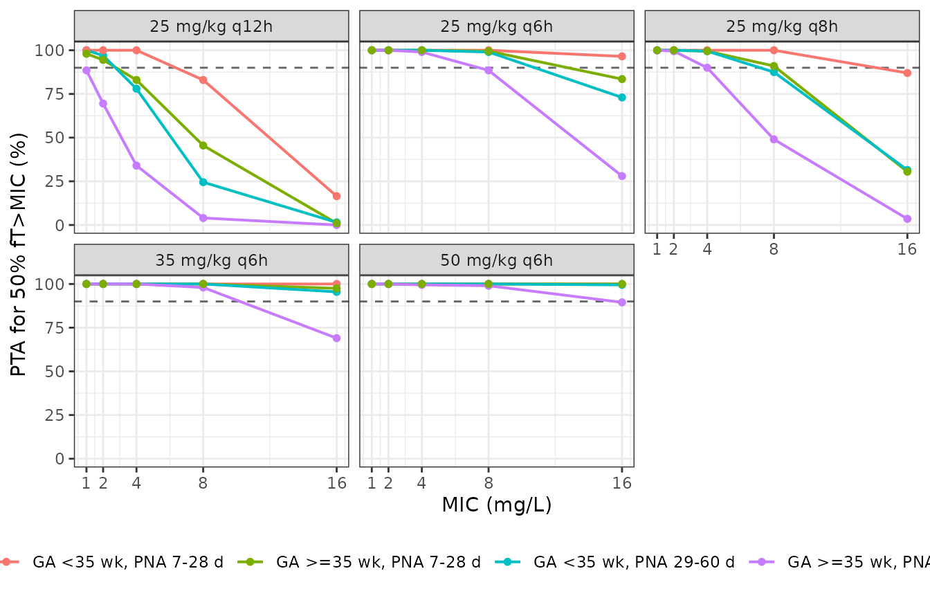
PTA for the 50% fT>MIC target across MICs, by regimen and stratum. Dashed line = the paper’s 90% goal.
What the PTA reproduction does and does not test
cell <- function(reg, a, mic, col) {
  v <- pta_tab[[col]][
    pta_tab$regimen == reg & pta_tab$arm == a & pta_tab$MIC == mic
  ]
  if (length(v) != 1L) {
    stop("no unique PTA row for '", reg, "' / '", a, "' at MIC ", mic)
  }
  v
}

least_mature <- arm_levels[1]  # GA <35 wk, PNA 7-28 d
most_mature <- arm_levels[4]   # GA >=35 wk, PNA 29-60 d
all_regimens <- sprintf("%g mg/kg q%gh", regimens$dose_mg_kg, regimens$tau)
stopifnot(all(all_regimens %in% pta_tab$regimen))

# 1. PTA must fall as MIC rises. Trend across the range, not step-by-step, so
#    a flat pair in the middle cannot flip the gate.
for (reg in all_regimens) {
  for (a in arm_levels) {
    s <- pta_tab |> filter(regimen == reg, arm == a) |> arrange(MIC)
    stopifnot(nrow(s) == length(mics))
    stopifnot(s$`PTA 50% (%)`[nrow(s)] <= s$`PTA 50% (%)`[1])
  }
}

# 2. The paper's central finding: more mature infants clear cephalexin faster
#    (CL/F scales with PMA^2.92), so they need MORE intensive dosing. At a
#    fixed regimen and a demanding MIC, PTA must be materially lower in the
#    most mature stratum than in the least mature one. Asserted as a magnitude
#    with headroom, not a bare ordering.
maturation_gaps <- c(
  q12_mic4 = cell("25 mg/kg q12h", least_mature, 4, "PTA 50% (%)") -
    cell("25 mg/kg q12h", most_mature, 4, "PTA 50% (%)"),
  q8_mic8 = cell("25 mg/kg q8h", least_mature, 8, "PTA 50% (%)") -
    cell("25 mg/kg q8h", most_mature, 8, "PTA 50% (%)")
)
maturation_gaps
#> q12_mic4  q8_mic8
#>     62.5     44.0
# Measured 66.0 / 66.0 (q12h at MIC 4) and 51.0 / 49.0 (q8h at MIC 8) at 2 and
# 8 solver threads: the effect is an order of magnitude larger than the bound.
stopifnot(all(maturation_gaps > 10))

# 3. Shortening the interval at a fixed mg/kg dose must raise PTA, and raising
#    the mg/kg dose at a fixed interval must raise PTA.
q_ladder <- vapply(
  c("25 mg/kg q12h", "25 mg/kg q8h", "25 mg/kg q6h"),
  function(r) cell(r, most_mature, 8, "PTA 50% (%)"), numeric(1)
)
d_ladder <- vapply(
  c("25 mg/kg q6h", "35 mg/kg q6h", "50 mg/kg q6h"),
  function(r) cell(r, most_mature, 16, "PTA 70% (%)"), numeric(1)
)
q_ladder
#> 25 mg/kg q12h  25 mg/kg q8h  25 mg/kg q6h
#>           5.5          56.0          89.0
d_ladder
#> 25 mg/kg q6h 35 mg/kg q6h 50 mg/kg q6h
#>          5.0         22.5         42.0
stopifnot(q_ladder[[3]] > q_ladder[[1]] + 10)
stopifnot(d_ladder[[3]] > d_ladder[[1]] + 10)

# 4. The regimens Table 3 recommends must clear a high PTA in the
#    corresponding stratum at an MIC inside the relevant range. MSSA
#    cephalexin MICs are "typically 1-4 mg/L" (Methods), and Table 3
#    recommends 25 mg/kg q12h for MSSA in both 7-28 day strata.
#    MIC 4 is the TOP of the MSSA range, so it is the hardest case the
#    recommendation has to cover; Table 3's CFR averages over 1-4 mg/L and is
#    correspondingly higher.
mssa_q12 <- c(
  cell("25 mg/kg q12h", arm_levels[1], 4, "PTA 50% (%)"),
  cell("25 mg/kg q12h", arm_levels[2], 4, "PTA 50% (%)")
)
mssa_q12
#> [1] 97.5 91.5
# Measured 100.0 / 97.0 (arm 1) and 83.0 / 87.0 (arm 2) at 2 and 8 solver
# threads. The binding value is ~83, and the binomial standard error of a
# proportion at n = 200 is ~2.6 points, so 80 would sit inside the noise.
# 70 keeps >= 13 points of headroom while still going red if clearance, dose
# or an exponent is mis-transcribed (those move PTA by 30-60 points, as the
# maturation gap above shows).
stopifnot(all(mssa_q12 >= 70))

# Table 3 recommends 25 mg/kg q8h (not q12h) for MSSA in the most mature
# stratum; both halves of that statement are checked. Measured 90.0 / 93.5 at
# 2 and 8 threads for q8h, against 34.0 / 31.0 for q12h.
stopifnot(cell("25 mg/kg q8h", most_mature, 4, "PTA 50% (%)") >= 75)
stopifnot(
  cell("25 mg/kg q8h", most_mature, 4, "PTA 50% (%)") >
    cell("25 mg/kg q12h", most_mature, 4, "PTA 50% (%)") + 10
)
The bounds above are deliberately loose relative to the values
printed in the tables: they are chosen to survive a different cohort
draw – rxSetSeed() fixes rxode2’s stream per solver thread,
not across thread counts, so CI draws a different cohort than a
developer does – while still failing on a mis-transcribed clearance,
dose, exponent or unit, all of which move PTA by far more than the
headroom allowed. Each bound was set after measuring the cell it guards
at two different solver-thread counts; the observed pairs are recorded
in the comments next to each assertion so a later reader does not
tighten them back into the noise. The threshold assertions carry at
least 13 percentage points of headroom against a binomial standard error
of about 2.6 points at 200 subjects per arm.
What is not reproduced here is the CFR column of Table 3 itself, because the MIC distributions it averages over are in an inaccessible appendix. The qualitative pattern of Table 3 – more frequent dosing needed as infants mature, and higher doses needed at the 16 mg/L Enterobacterales breakpoint – is what the gates above pin down.
Assumptions and deviations
-
Source is the peer-reviewed paper, not the conference abstract. This extraction started from IDWeek 2024 abstract P-1222 (Open Forum Infect Dis 2025;12(Suppl 1):S781, doi:10.1093/ofid/ofae631.1404, PMC11777916), which describes the same study but reports no parameter values at all. The peer-reviewed publication (J Pediatric Infect Dis Soc 2025;14(10):piaf088, PMC12551457) was located and used instead. The two differ materially, and every value here is the final published one:
Abstract (2024) Paper (2025, used here) Subjects / concentrations 27 / 114 33 / 144 Age range in title 0-60 days 7-60 days Covariate on CL/F eGFR postmenstrual age Protein binding 15% 10% Primary PD target 40% and 70% fT>MIC 50% fT>MIC (70% secondary) Omega scale. Table 2’s random-effect
Valuecolumn is read as a log-scale SD and squared to a variance forini(). This is confirmed arithmetically against the printedC.V.(%)column in the Omega scale section above, not assumed.PNA unit reparameterisation. The canonical
PNAcovariate column is carried in months (inst/references/covariate-columns.md), while the paper’s absorption equation is written in days with a 29.14-day reference.model()recovers days asPNA * 30.4375so the paper’s constant appears verbatim in the source.PAGEis carried in weeks, which the register permits when the source equations are written in weeks, matching the 41.06-week reference.No IIV on Vd/F. The authors did not estimate one, “due to high eta shrinkage and imprecise eta estimation” (Results, “Final Model”), so none is encoded. Simulated Vd/F therefore varies only with body weight.
No bioavailability parameter. All study doses were enteral and the paper reports apparent parameters (
CL/F,Vd/F), soFis not identifiable and is not encoded. Doses passed to this model are total administered amounts.Route is pooled. 20 of 33 infants were dosed through a gastric tube and 3 through a post-pyloric tube rather than by mouth. Route of administration was screened as a covariate and not retained, so one absorption model applies to all enteral routes – the authors’ own choice, and the reason they use “oral” throughout for all enteral routes.
Virtual cohort is reconstructed, not copied. The paper’s PTA simulations used a 20,000-subject PK-Sim population whose weight / GA / PNA distributions are in Figure S1, which is not in the accessible portion of the record. The cohort here is built from a documented birth-weight-for-GA approximation plus ~25 g/day postnatal weight gain and a 12% lognormal CV, sized at 200 per stratum. Absolute PTA values therefore differ from the paper’s; the gates assert the structural relationships instead.
Cohort assertions use centre and robust quantiles. Per this repository’s convention, assertions over a simulated cohort are made on medians and robust quantiles rather than extremes, because the extreme of a random cohort is not reproducible across rxode2 builds and thread counts. The two deterministic gates (closed form, typical-value NCA) are asserted tightly because they involve no random draws.
Steady-state window. PTA is computed over 24-48 h after the first dose, as the paper does. The paper notes first-interval PTAs were within 2 percentage points of steady state for MICs 1-8 mg/L, so the choice of window matters little below the top MIC.
Serum creatinine units. Recorded as mg/dL in
covariatesDataExcludedbecause the source does not state the unit; mg/dL is the conventional US reporting unit for the study site. This covariate is not used by the model.
Errata and record gaps
No erratum or correction to Haynes 2025 was found.
The record for this article is an NIH-funded author manuscript in Europe PMC (PMC12551457) rather than a fully open-access deposit. Consequences for this extraction:
- The main text and Tables 1-3 are complete and were used in
full. Every
ini()value, every structural equation and every reference constant comes from them. - Appendices A-C and Tables/Figures S1-S9 are not accessible. These hold the sampling protocol detail (A), the model-development narrative and covariate-selection table S3 (B), MIC distributions (C), the PK-Sim population distributions (S1), individual profiles and a VPC (S2-S3), ka-vs-PNA and CL-vs-PMA plots (S4-S5) and the full PTA/CFR surfaces (S6-S9). None of them contains a final parameter value that is absent from the main text, so the model is complete as encoded; what they would add is independent diagnostic confirmation and the MIC distributions needed to reproduce the CFR column of Table 3 exactly.