Imipenem and relebactam in HABP/VABP (Patel 2022)
Source:vignettes/articles/Patel_2022_imipenem_relebactam.Rmd
Patel_2022_imipenem_relebactam.RmdPatel M, Bellanti F, Daryani NM, Noormohamed N, Hilbert DW, Young K, Kulkarni P, Copalu W, Gheyas F, Rizk ML (2022). Population pharmacokinetic/ pharmacodynamic assessment of imipenem/cilastatin/relebactam in patients with hospital-acquired/ventilator-associated bacterial pneumonia. Clin Transl Sci 15(2):396-408. doi:10.1111/cts.13158. PMCID PMC8841461.
Patel 2022 updated the Bhagunde 2019 imipenem and relebactam
population PK models (see the
Bhagunde_2019_imipenem_relebactam article) with data from
the phase III RESTORE-IMI 2 study (PN014; hospital-acquired and
ventilator-associated bacterial pneumonia, HABP/VABP) and the Japanese
phase III study PN017. As in Bhagunde 2019, both analytes were fitted in
a single NONMEM run that switched on a DRUG flag, with no
shared parameter, random effect or residual term. The final control
stream is embedded in the supplement as finalmodel.txt
(Supplementary Methods, “Final Model”), and it confirms that the final
model has no imipenem-relebactam covariance; that term appears only in
the alternative model of Table S4. This package therefore carries the
analytes as two model files, validated together here:
Patel_2022_imipenemPatel_2022_relebactam
imi <- nlmixr2lib::modellib("Patel_2022_imipenem")
rel <- nlmixr2lib::modellib("Patel_2022_relebactam")

imi_ui <- rxode2::rxode2(imi)
rel_ui <- rxode2::rxode2(rel)
Population
The final dataset held 1,197 participants from 12 studies: the 855 of the Bhagunde 2019 analysis plus 261 from PN014 and 81 from PN017. Together they provided 6,100 quantifiable imipenem and 6,531 quantifiable relebactam concentrations (Results, “Analysis”). Participants were 18-96 years old (median 55) and weighed 27-180 kg (median 75). Cockcroft-Gault creatinine clearance ranged from 8 to 452 mL/min (median 106). 38.8% were female and 78.8% White; 10.3% were Japanese. By infection type there were 231 healthy participants (19.3%), 308 with complicated intra-abdominal infection (cIAI, 25.7%), 380 with complicated urinary tract infection (cUTI, 31.7%) and 278 with pneumonia (23.2%). Of the 261 PN014 pneumonia participants, 139 had nonventilated HABP, 30 ventilated HABP and 92 VABP (Table 2).
str(rxode2::modelExtract(imi, "population"), max.level = 1)
#>  chr(0)
Source trace
| Quantity | Imipenem | Relebactam | Source |
|---|---|---|---|
| Structure | 2-cmt IV, zero-order infusion, first-order elimination | same | Results, “Base model”; control stream
ADVAN3 TRANS4
|
lcl |
log(12.68 L/h) | log(7.23 L/h) | Table 3 footnote c (table body 12.7 / 7.23) |
lvc |
log(11.39 L) | log(11.21 L) | Table 3 footnote c (table body 11.4 / 11.2) |
lvp |
log(7.79 L) | log(6.15 L) | Table 3 footnote c |
lq |
log(23.07 L/h) | log(10.93 L/h) | Table 3 footnote c (table body 23.1 / 10.9) |
e_crcl_cl |
0.48 | 0.75 | Table 3, “Covariates on CL / CrCl (power)” |
e_wt_cl |
0.29 | not in model | Table 3 (relebactam NA); control stream
TVCL_RL = THETA(5)
|
e_habp_vabp_cl |
-0.38 | -0.43 | Table 3, “Covariates on CL / Pneumonia” |
e_wt_vc |
1.03 | 0.65 | Table 3, “Covariates on V1 / WT (power)” |
e_habp_vabp_vc |
-0.39 | -0.29 | Table 3, “Covariates on V1 / Pneumonia” |
e_mech_vent_vc |
+0.23 | +0.36 | Table 3, “Covariates on V1 / Ventilation”; control stream
THETA(16), THETA(15)
|
| CrCl / WT centring | 105.5 mL/min / 75 kg | same | Table 3 footnote c; control stream (CRCL/105.5),
(WT/75)
|
| Pneumonia reference | healthy + cIAI + cUTI | same | Table 3 footnote f; control stream INFC2 0/1/2 vs
3 |
| Ventilation reference | nonventilated pneumonia | same | Table 3 footnote g; control stream VENT2
|
etalcl |
0.530^2 | 0.436^2 | Table 3, “BSV in CL”, footnote h |
etalvc |
0.863^2 | 0.561^2 | Table 3, “BSV in V1”, footnote h |
etalvp |
0.635^2 | 0.587^2 | Table 3, “BSV in V2”, footnote h |
corr(etalcl, etalvc) |
0.97 | 0.62 | Table 3, “Corr CL ~ V1”, footnote i |
| BSV on Q | none | none | control stream $OMEGA 0 FIX ; [BSV_Q_IP] /
[BSV_Q_RL]
|
propSd |
0.295 | 0.226 | Table 3, “Residual error, proportional” |
| Additive residual | zero | zero | control stream $SIGMA 0 FIX
|
Table 3 footnote h gives the variability scale as
%CV = sqrt(omega^2) x 100, so
omega^2 = (CV/100)^2 directly, not the log-normal
log(CV^2 + 1). The control stream’s $OMEGA and
$SIGMA values are initial estimates seeded from a
near-final run: its $THETA values (for example 13.439 for
imipenem CL) differ from Table 3, so they are not the final estimates.
They still arbitrate the scale:
cs_var <- c(
  BSV_CL_IP = 0.281, BSV_V1_IP = 0.690, BSV_V2_IP = 0.443,
  BSV_CL_RL = 0.188, BSV_V1_RL = 0.312, BSV_V2_RL = 0.345,
  RES_prop_IP = 0.086, RES_prop_RL = 0.050
)
table3_cv <- c(
  BSV_CL_IP = 53.0, BSV_V1_IP = 86.3, BSV_V2_IP = 63.5,
  BSV_CL_RL = 43.6, BSV_V1_RL = 56.1, BSV_V2_RL = 58.7,
  RES_prop_IP = 29.5, RES_prop_RL = 22.6
)
data.frame(
  `control stream` = cs_var,
  `sqrt x 100` = round(sqrt(cs_var) * 100, 1),
  `log-normal CV` = round(sqrt(exp(cs_var) - 1) * 100, 1),
  `Table 3` = table3_cv,
  check.names = FALSE
) |>
  knitr::kable(caption = paste(
    "Control-stream variances against Table 3 under the footnote-h reading",
    "(sqrt x 100) and under the log-normal conversion."
))| control stream | sqrt x 100 | log-normal CV | Table 3 | |
|---|---|---|---|---|
| BSV_CL_IP | 0.281 | 53.0 | 57.0 | 53.0 |
| BSV_V1_IP | 0.690 | 83.1 | 99.7 | 86.3 |
| BSV_V2_IP | 0.443 | 66.6 | 74.7 | 63.5 |
| BSV_CL_RL | 0.188 | 43.4 | 45.5 | 43.6 |
| BSV_V1_RL | 0.312 | 55.9 | 60.5 | 56.1 |
| BSV_V2_RL | 0.345 | 58.7 | 64.2 | 58.7 |
| RES_prop_IP | 0.086 | 29.3 | 30.0 | 29.5 |
| RES_prop_RL | 0.050 | 22.4 | 22.6 | 22.6 |
# Arithmetic on published numbers: the footnote-h reading must beat the
# log-normal reading for every BSV entry. The two residual rows are shown for
# completeness only: a proportional-error SIGMA is a variance of a fractional
# error, so sqrt(SIGMA) is its SD whatever the omega convention, and at
# variances of 0.05-0.09 the two readings differ by under half a point anyway.
bsv <- grepl("^BSV", names(cs_var))
stopifnot(
  sum(bsv) == 6L,
  all(abs(sqrt(cs_var[bsv]) * 100 - table3_cv[bsv]) <
    abs(sqrt(exp(cs_var[bsv]) - 1) * 100 - table3_cv[bsv])),
  all(abs(sqrt(cs_var[!bsv]) * 100 - table3_cv[!bsv]) < 0.5)
)
A sign conflict in the Table 3 footnote
Table 3 footnote c writes the imipenem V1 equation with
(1+(Flag -0.23 Ventilation)), a minus sign, while the
relebactam equation has (1+(Flag x 0.36 Ventilation)). The
same imipenem footnote also has two plain typesetting slips: a stray
Pneumonia exponent and +exp(eta2) in place of
x exp(eta2). The relebactam CL equation has a stray
x 0.75 after the CrCl term, although relebactam CL has no
weight term. Three independent printings put the imipenem ventilation
effect at a positive value: the Table 3 estimate (0.23, 95% CI 0.02 to
0.45), the bootstrap (0.24, 0.02 to 0.48), and the control stream
(V1_IPVENT2 = 1 + THETA(16) with initial estimate
+0.215). The model encodes +0.23.
Model parameters as loaded
theta_imi <- imi_ui$theta
theta_rel <- rel_ui$theta
print(round(theta_imi, 5))
#>            lcl            lvc            lvp             lq      e_crcl_cl
#>        2.54003        2.43274        2.05284        3.13853        0.48000
#>        e_wt_cl e_habp_vabp_cl        e_wt_vc e_habp_vabp_vc e_mech_vent_vc
#>        0.29000       -0.38000        1.03000       -0.39000        0.23000
#>         propSd
#>        0.29500
print(round(theta_rel, 5))
#>            lcl            lvc            lvp             lq      e_crcl_cl
#>        1.97824        2.41681        1.81645        2.39151        0.75000
#> e_habp_vabp_cl        e_wt_vc e_habp_vabp_vc e_mech_vent_vc         propSd
#>       -0.43000        0.65000       -0.29000        0.36000        0.22600
need_imi <- c(
  "lcl", "lvc", "lvp", "lq", "e_crcl_cl", "e_wt_cl", "e_habp_vabp_cl",
  "e_wt_vc", "e_habp_vabp_vc", "e_mech_vent_vc", "propSd"
)
need_rel <- setdiff(need_imi, "e_wt_cl")
stopifnot(
  all(need_imi %in% names(theta_imi)),
  all(need_rel %in% names(theta_rel)),
  !("e_wt_cl" %in% names(theta_rel))
)
stopifnot(
  abs(exp(theta_imi[["lcl"]]) - 12.68) < 5e-3,
  abs(exp(theta_imi[["lvc"]]) - 11.39) < 5e-3,
  abs(exp(theta_imi[["lvp"]]) - 7.79) < 5e-3,
  abs(exp(theta_imi[["lq"]]) - 23.07) < 5e-3,
  abs(exp(theta_rel[["lcl"]]) - 7.23) < 5e-3,
  abs(exp(theta_rel[["lvc"]]) - 11.21) < 5e-3,
  abs(exp(theta_rel[["lvp"]]) - 6.15) < 5e-3,
  abs(exp(theta_rel[["lq"]]) - 10.93) < 5e-3
)
# The CL-V1 correlation must round-trip from the encoded covariance.
om_imi <- imi_ui$omega
om_rel <- rel_ui$omega
stopifnot(
  abs(cov2cor(om_imi[c("etalcl", "etalvc"), c("etalcl", "etalvc")])[1, 2] - 0.97) < 1e-6,
  abs(cov2cor(om_rel[c("etalcl", "etalvc"), c("etalcl", "etalvc")])[1, 2] - 0.62) < 1e-6
)
Molar-unit bridge and unbound fractions
The control stream doses in nmol and observes nmol/L. The model files dose in mg and predict mg/L, which gives the same parameters because the model is linear with CL and V in L/h and L. Patel 2022 states its exposure thresholds in uM and its PK/PD targets as unbound concentrations (“adjusted for protein binding”), but prints neither the molar masses nor the unbound fractions. The unbound fractions below are from the predecessor analysis by the same sponsor (Bhagunde 2019, Methods, “Probability of target attainment simulations”).
mw_imi <- 299.35 # g/mol, imipenem
mw_rel <- 348.37 # g/mol, relebactam
fu_imi <- 0.80 # Bhagunde 2019
fu_rel <- 0.78 # Bhagunde 2019
to_uM <- function(mg_per_L, mw) mg_per_L / mw * 1000
Typical-value profiles at the clinical dose
The clinical regimen is imipenem/cilastatin/relebactam 500/500/250 mg every 6 hours as a 30-minute infusion at CrCl >= 90 mL/min (Table S2). The typical profiles below are for a nonventilated pneumonia patient at the centring values, CrCl 105.5 mL/min and 75 kg.
tau <- 6
tinf <- 0.5
n_dose <- 40 # 10 days of q6h dosing; see Assumptions
t_last <- (n_dose - 1) * tau
grid_ss <- seq(t_last, t_last + tau, by = 0.05)

make_events <- function(ids, amt, covs, obs_times) {
  if (length(amt) == 1L) amt <- rep(amt, length(ids))
  dose <- data.frame(
    id = rep(ids, each = n_dose),
    time = rep(seq(0, by = tau, length.out = n_dose), times = length(ids)),
    amt = rep(amt, each = n_dose),
    evid = 1L,
    cmt = "central"
  )
  dose$rate <- dose$amt / tinf
  obs <- data.frame(
    id = rep(ids, each = length(obs_times)),
    time = rep(obs_times, times = length(ids)),
    amt = NA_real_,
    evid = 0L,
    # Observations point at the ODE state; rxode2 returns Cc as a column.
    cmt = "central",
    rate = NA_real_
  )
  out <- rbind(dose, obs)
  out <- out[order(out$id, out$time, -out$evid), ]
  merge(out, covs, by = "id", sort = FALSE)
}

covs_ref <- data.frame(
  id = 1L, CRCL = 105.5, WT = 75, DIS_HABP = 1, DIS_VABP = 0, MECH_VENT = 0
)
obs_typ <- sort(unique(c(seq(0, t_last, by = 0.25), grid_ss)))

typ_imi <- rxode2::rxSolve(
  rxode2::zeroRe(imi), make_events(1L, 500, covs_ref, obs_typ),
  returnType = "data.frame"
)
typ_rel <- rxode2::rxSolve(
  rxode2::zeroRe(rel), make_events(1L, 250, covs_ref, obs_typ),
  returnType = "data.frame"
)
stopifnot(nrow(typ_imi) > 0, nrow(typ_rel) > 0)
dplyr::bind_rows(
  typ_imi |> dplyr::mutate(Analyte = "Imipenem 500 mg"),
  typ_rel |> dplyr::mutate(Analyte = "Relebactam 250 mg")
) |>
  dplyr::filter(time >= t_last) |>
  dplyr::mutate(time = time - t_last) |>
  ggplot2::ggplot(ggplot2::aes(time, Cc, colour = Analyte)) +
  ggplot2::geom_line(linewidth = 0.8) +
  ggplot2::labs(
    x = "Time within the dosing interval (h)",
    y = "Plasma concentration (mg/L)", colour = NULL
  ) +
  ggplot2::theme_bw()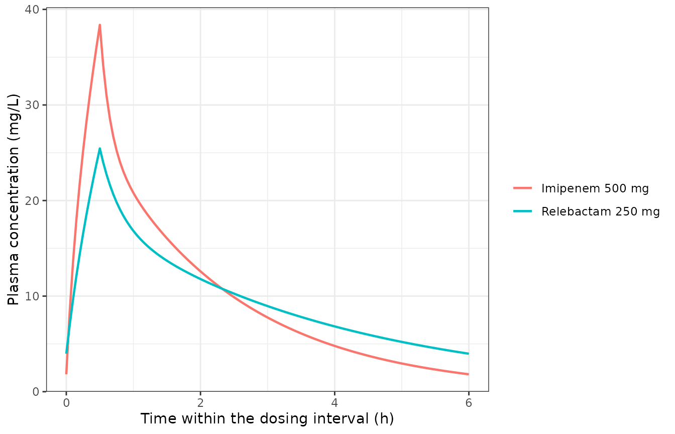
Typical steady-state profiles over the final 6-hour interval at imipenem/relebactam 500/250 mg q6h (30-minute infusion) in a nonventilated pneumonia patient, CrCl 105.5 mL/min, 75 kg.
An independent closed form
The two-compartment zero-order-infusion solution, superposed over the dosing history, is a reference that shares no code with the ODE solve. The typical parameters of the reference patient follow directly from Table 3 footnote c with the pneumonia factors applied.
cf_coef <- function(cl, vc, vp, q) {
  k10 <- cl / vc
  k12 <- q / vc
  k21 <- q / vp
  a1 <- k10 + k12 + k21
  a0 <- k10 * k21
  alpha <- (a1 + sqrt(a1^2 - 4 * a0)) / 2
  beta <- (a1 - sqrt(a1^2 - 4 * a0)) / 2
  list(
    alpha = alpha, beta = beta,
    A = (alpha - k21) / (vc * (alpha - beta)),
    B = (k21 - beta) / (vc * (alpha - beta)),
    cl = cl
  )
}
cf_one <- function(t, amt, cf) {
  r0 <- amt / tinf
  tin <- pmin(pmax(t, 0), tinf)
  ta <- pmax(t - tinf, 0)
  during <- cf$A / cf$alpha * (1 - exp(-cf$alpha * tin)) * exp(-cf$alpha * ta) +
    cf$B / cf$beta * (1 - exp(-cf$beta * tin)) * exp(-cf$beta * ta)
  ifelse(t <= 0, 0, r0 * during)
}
cf_multi <- function(t, amt, cf) {
  rowSums(vapply(
    seq_len(n_dose) - 1L,
    function(i) cf_one(t - i * tau, amt, cf),
    numeric(length(t))
  ))
}

cl_imi_ref <- 12.68 * (1 - 0.38)
cl_rel_ref <- 7.23 * (1 - 0.43)
cf_imi <- cf_coef(cl_imi_ref, 11.39 * (1 - 0.39), 7.79, 23.07)
cf_rel <- cf_coef(cl_rel_ref, 11.21 * (1 - 0.29), 6.15, 10.93)

# Instrument check: a very long infusion plateaus at R0 / CL.
stopifnot(
  abs(cf_imi$A / cf_imi$alpha + cf_imi$B / cf_imi$beta - 1 / cf_imi$cl) < 1e-10,
  abs(cf_rel$A / cf_rel$alpha + cf_rel$B / cf_rel$beta - 1 / cf_rel$cl) < 1e-10
)
cmp_cf <- function(sim, amt, cf) {
  d <- sim[sim$time >= t_last, ]
  ref <- cf_multi(d$time, amt, cf)
  max(abs(d$Cc - ref) / pmax(ref, 1e-8))
}
dev <- c(imipenem = cmp_cf(typ_imi, 500, cf_imi), relebactam = cmp_cf(typ_rel, 250, cf_rel))
dev
#>     imipenem   relebactam
#> 2.018402e-06 2.324047e-06
# Same parameters and dosing on both sides, so the only difference is
# integration error: about 2e-6 relative, at the solver's default relative
# tolerance of 1e-6. A tight bound is correct here; 1e-4 leaves room for that
# tolerance and still catches a wrong micro-constant, covariate factor or
# infusion rate, each of which moves the profile by well over 1e-3.
stopifnot(all(dev < 1e-4))
Covariate effects (Results, “Final model”)
The paper reports the simulated AUC0-24 fold changes for
its Table 1 scenarios, all relative to patients with normal renal
function (CrCl 90-150 mL/min) weighing 70-90 kg. Healthy participants
had fold changes of 0.62 (imipenem) and 0.57 (relebactam) against
pneumonia patients at the same weight and renal function. AUC was
similar in ventilated and nonventilated patients, because ventilation
acts on V1 only.
typ_auc <- function(mod, amt, covs) {
  s <- rxode2::rxSolve(
    rxode2::zeroRe(mod), make_events(1L, amt, covs, grid_ss),
    returnType = "data.frame"
  )
  c(
    auc = sum(diff(s$time) * (head(s$Cc, -1) + tail(s$Cc, -1)) / 2),
    cmax = max(s$Cc)
  )
}
cov_healthy <- transform(covs_ref, DIS_HABP = 0)
cov_vent <- transform(covs_ref, DIS_HABP = 0, DIS_VABP = 1, MECH_VENT = 1)
cov_vent_habp <- transform(covs_ref, MECH_VENT = 1)
cov_vent_nonpneu <- transform(covs_ref, DIS_HABP = 0, MECH_VENT = 1)

eff <- tibble::tibble(
  Analyte = c("Imipenem", "Relebactam"),
  `Healthy / pneumonia AUC (sim)` = c(
    typ_auc(imi, 500, cov_healthy)[["auc"]] / typ_auc(imi, 500, covs_ref)[["auc"]],
    typ_auc(rel, 250, cov_healthy)[["auc"]] / typ_auc(rel, 250, covs_ref)[["auc"]]
  ),
  `Healthy / pneumonia AUC (paper)` = c(0.62, 0.57),
  `Ventilated / nonventilated AUC` = c(
    typ_auc(imi, 500, cov_vent)[["auc"]] / typ_auc(imi, 500, covs_ref)[["auc"]],
    typ_auc(rel, 250, cov_vent)[["auc"]] / typ_auc(rel, 250, covs_ref)[["auc"]]
  ),
  `Ventilated / nonventilated Cmax` = c(
    typ_auc(imi, 500, cov_vent)[["cmax"]] / typ_auc(imi, 500, covs_ref)[["cmax"]],
    typ_auc(rel, 250, cov_vent)[["cmax"]] / typ_auc(rel, 250, covs_ref)[["cmax"]]
  )
)
knitr::kable(eff, digits = 3)| Analyte | Healthy / pneumonia AUC (sim) | Healthy / pneumonia AUC (paper) | Ventilated / nonventilated AUC | Ventilated / nonventilated Cmax |
|---|---|---|---|---|
| Imipenem | 0.62 | 0.62 | 1 | 0.914 |
| Relebactam | 0.57 | 0.57 | 1 | 0.858 |
stopifnot(
  all(abs(eff$`Healthy / pneumonia AUC (sim)` / eff$`Healthy / pneumonia AUC (paper)` - 1) < 0.01),
  all(abs(eff$`Ventilated / nonventilated AUC` - 1) < 0.002),
  all(eff$`Ventilated / nonventilated Cmax` < 1)
)
# Ventilated HABP and VABP are the same stratum, and ventilation outside
# pneumonia has no effect (Table 3 footnote g).
stopifnot(
  abs(typ_auc(imi, 500, cov_vent_habp)[["cmax"]] / typ_auc(imi, 500, cov_vent)[["cmax"]] - 1) < 1e-8,
  abs(typ_auc(rel, 250, cov_vent_nonpneu)[["cmax"]] / typ_auc(rel, 250, cov_healthy)[["cmax"]] - 1) < 1e-8
)
Renal-impairment fold changes
The renal fold changes were 1.23, 1.59 and 2.18 (imipenem) and 1.39,
2.05 and 3.35 (relebactam) for mild, moderate and severe impairment. The
paper does not print the CrCl values it simulated at. Because both
analytes carry a pure power term in CrCl and the same weight band, each
imipenem ratio fixes an effective CrCl ratio
ratio = fold^(1 / 0.48). That ratio then predicts the
relebactam ratio ratio^0.75 with no further information.
This is arithmetic on published numbers, and it tests both exponents at
once.
fold_pub <- tibble::tibble(
  group = c("Mild RI", "Moderate RI", "Severe RI"),
  crcl_lo = c(60, 30, 15),
  crcl_hi = c(90, 60, 30),
  imi = c(1.23, 1.59, 2.18),
  rel = c(1.39, 2.05, 3.35)
) |>
  dplyr::mutate(
    crcl_ratio = imi^(1 / 0.48),
    rel_pred = crcl_ratio^0.75,
    rel_dev_pct = 100 * (rel_pred / rel - 1),
    crcl_implied = 120 / crcl_ratio
  )
knitr::kable(
  fold_pub |> dplyr::rename(
    Group = group, `Imipenem fold` = imi, `Relebactam fold (paper)` = rel,
    `Relebactam fold (predicted)` = rel_pred, `Deviation (%)` = rel_dev_pct,
    `Implied CrCl at a 120 mL/min reference` = crcl_implied
  ) |> dplyr::select(-crcl_lo, -crcl_hi, -crcl_ratio),
  digits = 2
)| Group | Imipenem fold | Relebactam fold (paper) | Relebactam fold (predicted) | Deviation (%) | Implied CrCl at a 120 mL/min reference |
|---|---|---|---|---|---|
| Mild RI | 1.23 | 1.39 | 1.38 | -0.58 | 77.96 |
| Moderate RI | 1.59 | 2.05 | 2.06 | 0.68 | 45.67 |
| Severe RI | 2.18 | 3.35 | 3.38 | 0.88 | 23.66 |
# A swapped or mis-transcribed exponent moves these by tens of percent.
stopifnot(
  all(abs(fold_pub$rel_dev_pct) < 3),
  all(fold_pub$crcl_implied >= fold_pub$crcl_lo & fold_pub$crcl_implied < fold_pub$crcl_hi)
)
# The model files must implement the same power form: simulate the typical
# patient at CrCl 120 and at 120 / ratio.
sim_fold <- vapply(seq_len(nrow(fold_pub)), function(i) {
  lo <- transform(covs_ref, CRCL = fold_pub$crcl_implied[i])
  hi <- transform(covs_ref, CRCL = 120)
  c(
    imi = typ_auc(imi, 500, lo)[["auc"]] / typ_auc(imi, 500, hi)[["auc"]],
    rel = typ_auc(rel, 250, lo)[["auc"]] / typ_auc(rel, 250, hi)[["auc"]]
  )
}, numeric(2))
stopifnot(
  all(abs(sim_fold["imi", ] / fold_pub$imi - 1) < 0.005),
  all(abs(sim_fold["rel", ] / fold_pub$rel - 1) < 0.03)
)
PKNCA validation
conc_df <- dplyr::bind_rows(
  typ_imi |> dplyr::transmute(id = 1L, treatment = "Imipenem 500 mg q6h", time, Cc),
  typ_rel |> dplyr::transmute(id = 1L, treatment = "Relebactam 250 mg q6h", time, Cc)
) |>
  dplyr::filter(!is.na(Cc), time >= t_last)
dose_df <- data.frame(
  id = 1L,
  treatment = c("Imipenem 500 mg q6h", "Relebactam 250 mg q6h"),
  time = t_last,
  amt = c(500, 250)
)
nca_res <- PKNCA::pk.nca(PKNCA::PKNCAdata(
  PKNCA::PKNCAconc(conc_df, Cc ~ time | id / treatment),
  PKNCA::PKNCAdose(dose_df, amt ~ time | id + treatment),
  intervals = data.frame(
    start = t_last, end = t_last + tau,
    cmax = TRUE, cmin = TRUE, tmax = TRUE, auclast = TRUE, cav = TRUE
  )
))
Patel 2022 publishes no NCA table. The reference side is therefore
built from the published parameters. AUCtau comes from the
steady-state mass balance Dose / CL, Cav is
that AUC divided by the interval, and Cmax,
Cmin and Tmax come from the closed form.
ref_row <- function(label, amt, cf) {
  g <- seq(t_last, t_last + tau, by = 1e-3)
  cc <- cf_multi(g, amt, cf)
  tibble::tibble(
    treatment = label,
    auclast = amt / cf$cl,
    cav = amt / (cf$cl * tau),
    cmax = max(cc),
    cmin = min(cc),
    tmax = g[which.max(cc)] - t_last
  )
}
published <- dplyr::bind_rows(
  ref_row("Imipenem 500 mg q6h", 500, cf_imi),
  ref_row("Relebactam 250 mg q6h", 250, cf_rel)
)
cmp <- nlmixr2lib::ncaComparisonTable(
  simulated = nca_res,
  reference = published,
  by = "treatment",
  units = c(auclast = "mg*h/L", cav = "mg/L", cmax = "mg/L", cmin = "mg/L", tmax = "h"),
  tolerance_pct = 20
)
knitr::kable(
  cmp,
  caption = paste(
    "Steady-state NCA of the typical nonventilated pneumonia patient against",
    "values derived from Patel 2022 Table 3. * differs by >20%."
  ),
  align = c("l", "l", "r", "r", "r")
)| NCA parameter | treatment | Reference | Simulated | % diff |
|---|---|---|---|---|
| Cmax (mg/L) | Imipenem 500 mg q6h | 38.4 | 38.4 | +0.0% |
| Cmax (mg/L) | Relebactam 250 mg q6h | 25.5 | 25.5 | +0.0% |
| Cmin (mg/L) | Imipenem 500 mg q6h | 1.82 | 1.82 | -0.0% |
| Cmin (mg/L) | Relebactam 250 mg q6h | 3.97 | 3.97 | +0.0% |
| Tmax (h) | Imipenem 500 mg q6h | 0.5 | 0.5 | +0.0% |
| Tmax (h) | Relebactam 250 mg q6h | 0.5 | 0.5 | +0.0% |
| AUClast (mg*h/L) | Imipenem 500 mg q6h | 63.6 | 63.6 | -0.0% |
| AUClast (mg*h/L) | Relebactam 250 mg q6h | 60.7 | 60.7 | -0.0% |
| Cavg (mg/L) | Imipenem 500 mg q6h | 10.6 | 10.6 | -0.0% |
| Cavg (mg/L) | Relebactam 250 mg q6h | 10.1 | 10.1 | -0.0% |
nca_val <- function(trt, param) {
  v <- nca_res$result$PPORRES[
    nca_res$result$treatment == trt & nca_res$result$PPTESTCD == param
  ]
  if (length(v) != 1L) stop("no unique ", param, " for '", trt, "'")
  v
}
stopifnot(
  abs(nca_val("Imipenem 500 mg q6h", "auclast") / (500 / cl_imi_ref) - 1) < 0.005,
  abs(nca_val("Relebactam 250 mg q6h", "auclast") / (250 / cl_rel_ref) - 1) < 0.005,
  abs(nca_val("Imipenem 500 mg q6h", "cmax") / published$cmax[1] - 1) < 0.02,
  abs(nca_val("Relebactam 250 mg q6h", "cmax") / published$cmax[2] - 1) < 0.02
)
Joint probability of target attainment (Figure 2, Tables S5 and S6)
Joint attainment requires both targets. For imipenem the target is
30% (40% in the sensitivity analysis) of the dosing interval with
unbound concentration above the MIC. For relebactam it is
fAUC0-24/MIC >= 8, with the MIC being that of imipenem
in the presence of a fixed 4 ug/mL relebactam. Doses follow the Table S3
renal categories.
The paper sampled its virtual patients from the PN014 pneumonia population, with ESRD patients taken from the MODIFY I/II studies. It drew them from a 1,000,000-patient set using the observed weight-CrCl variance-covariance. Those data are not published. The cohort below instead draws CrCl uniformly within each category and weight log-normally around 75 kg, independently of CrCl. It has 100 nonventilated (HABP) and 100 ventilated (VABP) patients per category.
rxode2::rxSetSeed(20220215)
set.seed(20220215)

n_per_arm <- 100L
bands <- tibble::tibble(
  band = c(
    "ESRD", "Severe RI", "Moderate RI", "Mild RI", "Normal",
    "ARC 150-180", "ARC 180-210", "ARC 210-250"
  ),
  crcl_lo = c(5, 15, 30, 60, 90, 150, 180, 210),
  crcl_hi = c(15, 30, 60, 90, 150, 180, 210, 250),
  imi_dose = c(200, 200, 300, 400, 500, 500, 500, 500),
  rel_dose = c(100, 100, 150, 200, 250, 250, 250, 250)
)

cohort <- tidyr::expand_grid(bands, vent = c("Nonventilated", "Ventilated")) |>
  dplyr::rowwise() |>
  dplyr::reframe(
    band = band, vent = vent, imi_dose = imi_dose, rel_dose = rel_dose,
    CRCL = runif(n_per_arm, crcl_lo, crcl_hi),
    WT = rlnorm(n_per_arm, log(75), 0.22)
  ) |>
  dplyr::mutate(
    id = dplyr::row_number(),
    DIS_HABP = as.numeric(vent == "Nonventilated"),
    DIS_VABP = as.numeric(vent == "Ventilated"),
    MECH_VENT = as.numeric(vent == "Ventilated")
  )
stopifnot(nrow(cohort) == n_per_arm * 2L * nrow(bands))
cov_cols <- c("id", "CRCL", "WT", "DIS_HABP", "DIS_VABP", "MECH_VENT")
sim_imi <- rxode2::rxSolve(
  imi, make_events(cohort$id, cohort$imi_dose, cohort[, cov_cols], grid_ss),
  returnType = "data.frame"
)
sim_rel <- rxode2::rxSolve(
  rel, make_events(cohort$id, cohort$rel_dose, cohort[, cov_cols], grid_ss),
  returnType = "data.frame"
)
stopifnot(
  nrow(sim_imi) == nrow(cohort) * length(grid_ss),
  nrow(sim_rel) == nrow(sim_imi),
  all(sim_imi$Cc >= 0), all(sim_rel$Cc >= 0)
)
Relebactam AUCtau is taken through PKNCA, one call per
renal category. Imipenem %fT>MIC is a
time-above-threshold statistic computed on the same dense grid.
rel_auc <- lapply(split(cohort, cohort$band), function(d) {
  conc <- sim_rel |>
    dplyr::filter(id %in% d$id, !is.na(Cc)) |>
    dplyr::mutate(treatment = d$band[1]) |>
    dplyr::select(id, treatment, time, Cc)
  dose <- d |> dplyr::transmute(id, treatment = band, time = t_last, amt = rel_dose)
  res <- PKNCA::pk.nca(PKNCA::PKNCAdata(
    PKNCA::PKNCAconc(conc, Cc ~ time | id / treatment),
    PKNCA::PKNCAdose(dose, amt ~ time | id + treatment),
    intervals = data.frame(start = t_last, end = t_last + tau, auclast = TRUE)
  ))
  res$result |>
    dplyr::filter(PPTESTCD == "auclast") |>
    dplyr::transmute(id, auc_tau = PPORRES)
}) |>
  dplyr::bind_rows()
stopifnot(nrow(rel_auc) == nrow(cohort))

# Fraction of the interval (%) with unbound imipenem above each MIC, under the
# Bhagunde 2019 unbound fraction (0.80) and, as a sensitivity reading, with no
# binding adjustment for imipenem (1.0); see the discussion below the table.
mic_grid <- c(0.5, 1, 2, 4, 8, 16, 32)
fu_imi_grid <- c(fu_imi, 1)
ft_above <- function(d, thr) {
  above <- d$Cc > thr
  100 * sum(diff(d$time) * (head(above, -1) + tail(above, -1)) / 2) / tau
}
imi_ft <- sim_imi |>
  dplyr::arrange(id, time) |>
  dplyr::group_by(id) |>
  dplyr::group_modify(function(d, key) {
    g <- expand.grid(mic = mic_grid, fu = fu_imi_grid)
    g$ft <- mapply(function(m, f) ft_above(d, m / f), g$mic, g$fu)
    tibble::as_tibble(g)
  }) |>
  dplyr::ungroup()

pta <- imi_ft |>
  dplyr::inner_join(rel_auc, by = "id") |>
  dplyr::inner_join(cohort[, c("id", "band", "vent")], by = "id") |>
  dplyr::mutate(
    rel_fauc_mic = fu_rel * (24 / tau) * auc_tau / mic,
    joint30 = ft >= 30 & rel_fauc_mic >= 8,
    joint40 = ft >= 40 & rel_fauc_mic >= 8
  )
stopifnot(nrow(pta) == nrow(cohort) * length(mic_grid) * length(fu_imi_grid))
# Table S6 (combined ventilation strata, 40% fT>MIC), columns MIC 2, 8, 16.
pub_s6 <- tibble::tribble(
  ~band, ~mic, ~pub,
  "ESRD", 2, 100, "ESRD", 8, 93.2, "ESRD", 16, 58.0,
  "Severe RI", 2, 100, "Severe RI", 8, 76.8, "Severe RI", 16, 29.4,
  "Moderate RI", 2, 100, "Moderate RI", 8, 76.6, "Moderate RI", 16, 30.2,
  "Mild RI", 2, 100, "Mild RI", 8, 75.2, "Mild RI", 16, 25.1,
  "Normal", 2, 100, "Normal", 8, 69.9, "Normal", 16, 20.4,
  "ARC 150-180", 2, 99.9, "ARC 150-180", 8, 50.4, "ARC 150-180", 16, 8.7,
  "ARC 180-210", 2, 99.4, "ARC 180-210", 8, 41.1, "ARC 180-210", 16, 4.7,
  "ARC 210-250", 2, 98.2, "ARC 210-250", 8, 33.2, "ARC 210-250", 16, 2.8
)
# Table S5 (30% fT>MIC), nonventilated and ventilated averaged, MIC 8 and 16.
pub_s5 <- tibble::tribble(
  ~band, ~mic, ~pub,
  "ESRD", 8, (94.8 + 94.8) / 2, "ESRD", 16, (65.6 + 64.8) / 2,
  "Severe RI", 8, (84.6 + 83.2) / 2, "Severe RI", 16, (35.4 + 34.4) / 2,
  "Moderate RI", 8, (85.4 + 83.8) / 2, "Moderate RI", 16, (39.6 + 37.4) / 2,
  "Mild RI", 8, (86.2 + 86.4) / 2, "Mild RI", 16, (35.2 + 35.4) / 2,
  "Normal", 8, (83.4 + 86.6) / 2, "Normal", 16, (30.4 + 31.4) / 2,
  "ARC 150-180", 8, (67.6 + 70.4) / 2, "ARC 150-180", 16, (14.6 + 17.0) / 2,
  "ARC 180-210", 8, (58.8 + 63.0) / 2, "ARC 180-210", 16, (10.4 + 11.0) / 2,
  "ARC 210-250", 8, (49.0 + 51.6) / 2, "ARC 210-250", 16, (6.6 + 5.6) / 2
)

sim_pta <- pta |>
  dplyr::group_by(fu, band, mic) |>
  dplyr::summarise(
    pta30 = 100 * mean(joint30),
    pta40 = 100 * mean(joint40),
    .groups = "drop"
  )
sim_wide <- sim_pta |>
  tidyr::pivot_wider(names_from = fu, values_from = c(pta30, pta40))
col_08 <- paste0("_", fu_imi)
cmp_pta <- dplyr::bind_rows(
  pub_s5 |> dplyr::mutate(target = "30% fT>MIC (Table S5)") |>
    dplyr::left_join(
      sim_wide |> dplyr::select(band, mic, sim08 = dplyr::all_of(paste0("pta30", col_08)), sim10 = pta30_1),
      by = c("band", "mic")
    ),
  pub_s6 |> dplyr::mutate(target = "40% fT>MIC (Table S6)") |>
    dplyr::left_join(
      sim_wide |> dplyr::select(band, mic, sim08 = dplyr::all_of(paste0("pta40", col_08)), sim10 = pta40_1),
      by = c("band", "mic")
    )
) |>
  dplyr::mutate(
    diff08 = sim08 - pub, diff10 = sim10 - pub,
    band = factor(band, levels = bands$band)
  ) |>
  dplyr::arrange(target, band, mic)
stopifnot(nrow(cmp_pta) == 40L, !anyNA(cmp_pta$sim08), !anyNA(cmp_pta$sim10))

knitr::kable(
  cmp_pta |>
    dplyr::rename(
      Target = target, `Renal category` = band, `MIC (ug/mL)` = mic,
      `Published (%)` = pub,
      `Simulated, imipenem fu 0.80 (%)` = sim08,
      `Difference, fu 0.80` = diff08,
      `Simulated, imipenem fu 1.0 (%)` = sim10,
      `Difference, fu 1.0` = diff10
    ),
  digits = 1,
  caption = paste(
    "Joint PTA by renal category against Tables S5 (ventilation strata",
    "averaged) and S6, at the MICs where attainment is not saturated.",
    "Differences are simulated minus published, in percentage points."
  )
)| Renal category | MIC (ug/mL) | Published (%) | Target | Simulated, imipenem fu 0.80 (%) | Simulated, imipenem fu 1.0 (%) | Difference, fu 0.80 | Difference, fu 1.0 |
|---|---|---|---|---|---|---|---|
| ESRD | 8 | 94.8 | 30% fT>MIC (Table S5) | 76.0 | 91.5 | -18.8 | -3.3 |
| ESRD | 16 | 65.2 | 30% fT>MIC (Table S5) | 27.5 | 47.0 | -37.7 | -18.2 |
| Severe RI | 8 | 83.9 | 30% fT>MIC (Table S5) | 56.5 | 71.0 | -27.4 | -12.9 |
| Severe RI | 16 | 34.9 | 30% fT>MIC (Table S5) | 12.0 | 21.5 | -22.9 | -13.4 |
| Moderate RI | 8 | 84.6 | 30% fT>MIC (Table S5) | 57.0 | 73.5 | -27.6 | -11.1 |
| Moderate RI | 16 | 38.5 | 30% fT>MIC (Table S5) | 12.5 | 20.5 | -26.0 | -18.0 |
| Mild RI | 8 | 86.3 | 30% fT>MIC (Table S5) | 65.0 | 78.0 | -21.3 | -8.3 |
| Mild RI | 16 | 35.3 | 30% fT>MIC (Table S5) | 14.0 | 26.5 | -21.3 | -8.8 |
| Normal | 8 | 85.0 | 30% fT>MIC (Table S5) | 61.0 | 75.0 | -24.0 | -10.0 |
| Normal | 16 | 30.9 | 30% fT>MIC (Table S5) | 14.5 | 24.0 | -16.4 | -6.9 |
| ARC 150-180 | 8 | 69.0 | 30% fT>MIC (Table S5) | 46.0 | 63.5 | -23.0 | -5.5 |
| ARC 150-180 | 16 | 15.8 | 30% fT>MIC (Table S5) | 5.5 | 9.5 | -10.3 | -6.3 |
| ARC 180-210 | 8 | 60.9 | 30% fT>MIC (Table S5) | 43.0 | 61.5 | -17.9 | 0.6 |
| ARC 180-210 | 16 | 10.7 | 30% fT>MIC (Table S5) | 4.5 | 6.0 | -6.2 | -4.7 |
| ARC 210-250 | 8 | 50.3 | 30% fT>MIC (Table S5) | 35.0 | 49.0 | -15.3 | -1.3 |
| ARC 210-250 | 16 | 6.1 | 30% fT>MIC (Table S5) | 1.5 | 4.5 | -4.6 | -1.6 |
| ESRD | 2 | 100.0 | 40% fT>MIC (Table S6) | 99.5 | 100.0 | -0.5 | 0.0 |
| ESRD | 8 | 93.2 | 40% fT>MIC (Table S6) | 71.0 | 85.5 | -22.2 | -7.7 |
| ESRD | 16 | 58.0 | 40% fT>MIC (Table S6) | 21.0 | 40.5 | -37.0 | -17.5 |
| Severe RI | 2 | 100.0 | 40% fT>MIC (Table S6) | 98.5 | 100.0 | -1.5 | 0.0 |
| Severe RI | 8 | 76.8 | 40% fT>MIC (Table S6) | 49.5 | 60.5 | -27.3 | -16.3 |
| Severe RI | 16 | 29.4 | 40% fT>MIC (Table S6) | 8.5 | 15.5 | -20.9 | -13.9 |
| Moderate RI | 2 | 100.0 | 40% fT>MIC (Table S6) | 100.0 | 100.0 | 0.0 | 0.0 |
| Moderate RI | 8 | 76.6 | 40% fT>MIC (Table S6) | 45.5 | 62.0 | -31.1 | -14.6 |
| Moderate RI | 16 | 30.2 | 40% fT>MIC (Table S6) | 9.0 | 15.5 | -21.2 | -14.7 |
| Mild RI | 2 | 100.0 | 40% fT>MIC (Table S6) | 99.5 | 100.0 | -0.5 | 0.0 |
| Mild RI | 8 | 75.2 | 40% fT>MIC (Table S6) | 49.5 | 66.5 | -25.7 | -8.7 |
| Mild RI | 16 | 25.1 | 40% fT>MIC (Table S6) | 7.0 | 14.5 | -18.1 | -10.6 |
| Normal | 2 | 100.0 | 40% fT>MIC (Table S6) | 98.5 | 100.0 | -1.5 | 0.0 |
| Normal | 8 | 69.9 | 40% fT>MIC (Table S6) | 38.5 | 55.5 | -31.4 | -14.4 |
| Normal | 16 | 20.4 | 40% fT>MIC (Table S6) | 6.5 | 13.0 | -13.9 | -7.4 |
| ARC 150-180 | 2 | 99.9 | 40% fT>MIC (Table S6) | 98.0 | 99.0 | -1.9 | -0.9 |
| ARC 150-180 | 8 | 50.4 | 40% fT>MIC (Table S6) | 26.5 | 40.0 | -23.9 | -10.4 |
| ARC 150-180 | 16 | 8.7 | 40% fT>MIC (Table S6) | 3.0 | 5.5 | -5.7 | -3.2 |
| ARC 180-210 | 2 | 99.4 | 40% fT>MIC (Table S6) | 97.5 | 99.5 | -1.9 | 0.1 |
| ARC 180-210 | 8 | 41.1 | 40% fT>MIC (Table S6) | 23.5 | 34.5 | -17.6 | -6.6 |
| ARC 180-210 | 16 | 4.7 | 40% fT>MIC (Table S6) | 1.0 | 4.5 | -3.7 | -0.2 |
| ARC 210-250 | 2 | 98.2 | 40% fT>MIC (Table S6) | 96.5 | 97.5 | -1.7 | -0.7 |
| ARC 210-250 | 8 | 33.2 | 40% fT>MIC (Table S6) | 17.0 | 27.5 | -16.2 | -5.7 |
| ARC 210-250 | 16 | 2.8 | 40% fT>MIC (Table S6) | 0.5 | 1.0 | -2.3 | -1.8 |
The simulation reproduces the headline result: joint attainment is
above 90% at the 2 ug/mL breakpoint in every renal category, and it
falls with rising CrCl in the same order as Tables S5 and S6. At MIC 8
and 16 ug/mL, where imipenem fT>MIC is the binding
target, the cells are not reproduced. With the imipenem unbound fraction
of 0.80 from Bhagunde 2019, simulated attainment runs about 20 points
below the published values. Without a binding adjustment for imipenem,
the median gap narrows to about 8 points. Relebactam reaches its target
in more than 75% of patients at 16 ug/mL outside the augmented-clearance
categories, so it does not drive these cells.
The transcription of the model is not the cause. The closed-form,
mass-balance and fold-change checks above pin the clearances, volumes
and covariate effects to Table 3 and the control stream. The difference
comes from simulation inputs the paper does not publish: the imipenem
unbound fraction it used, and its virtual cohort. The cohort matters
because the paper’s own safety simulation below yields 90th-percentile
Cmax values well above this cohort’s, which means more
peaked profiles and therefore more time above high MICs. The gates below
therefore assert the headline claim, the ordering across renal
categories and the fu = 1.0 reading, and the fu = 0.80 column is
reported without a gate.
# Headline claim: joint PTA > 90% at the 2 ug/mL breakpoint in every renal
# category, under both targets and both unbound-fraction readings.
stopifnot(
  all(sim_pta$pta30[sim_pta$mic == 2] > 90),
  all(sim_pta$pta40[sim_pta$mic == 2] > 90)
)
# The unsaturated cells under the fu = 1.0 reading. The cohort is a
# substitute for the paper's, so the check is on the centre of the per-cell
# differences and a robust envelope, never on one cell. Realised: median -8.5,
# 90th-percentile |difference| 16 points (binomial SE per cell about 3.5
# points at n = 200). A mis-transcribed clearance or dose moves the median by
# far more than 15.
unsat <- cmp_pta$mic > 2
stopifnot(
  abs(median(cmp_pta$diff10[unsat])) < 15,
  quantile(abs(cmp_pta$diff10[unsat]), 0.9) < 25
)
# A binding adjustment only lowers unbound exposure, so the fu = 0.80 column
# must sit below the fu = 1.0 column.
stopifnot(median(cmp_pta$sim08[unsat] - cmp_pta$sim10[unsat]) < 0)
# The published shape: attainment at MIC 16 falls from ESRD to the highest
# augmented-clearance category.
p16 <- sim_pta |> dplyr::filter(mic == 16, fu == fu_imi)
stopifnot(
  p16$pta30[p16$band == "ESRD"] > p16$pta30[p16$band == "Normal"],
  p16$pta30[p16$band == "Normal"] > p16$pta30[p16$band == "ARC 210-250"]
)
sim_pta |>
  dplyr::filter(fu == fu_imi) |>
  dplyr::mutate(band = factor(band, levels = bands$band)) |>
  ggplot2::ggplot(ggplot2::aes(mic, pta30, colour = band)) +
  ggplot2::geom_line(linewidth = 0.8) +
  ggplot2::geom_point() +
  ggplot2::geom_hline(yintercept = 90, linetype = "dashed") +
  ggplot2::geom_vline(xintercept = 2, linetype = "dotted") +
  ggplot2::scale_x_log10(breaks = mic_grid) +
  ggplot2::labs(x = "MIC (ug/mL)", y = "Joint PTA (%)", colour = "Renal category") +
  ggplot2::theme_bw()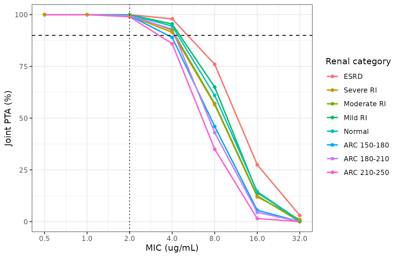
Joint PTA across MIC by renal category (30% fT>MIC for imipenem; relebactam fAUC0-24/MIC >= 8), under the Table S3 renal dose adjustments, with the imipenem unbound fraction 0.80; compare Figure 2a. The horizontal line is 90% attainment and the vertical line the 2 ug/mL breakpoint.
Ventilation status
Table S5 shows almost identical attainment for ventilated and nonventilated patients. Ventilation changes V1 only, which leaves AUC unchanged and alters only the shape of the profile.
vent_diff <- pta |>
  dplyr::filter(fu == fu_imi, mic %in% c(8, 16)) |>
  dplyr::group_by(band, mic, vent) |>
  dplyr::summarise(p = 100 * mean(joint30), .groups = "drop") |>
  tidyr::pivot_wider(names_from = vent, values_from = p) |>
  dplyr::mutate(diff = Ventilated - Nonventilated)
# Published ventilated-minus-nonventilated differences at MIC 8 and 16 span
# -2.6 to +4.2 points; at 100 patients per stratum the binomial standard error
# of a difference is up to 7 points, so only the centre is asserted.
stopifnot(abs(median(vent_diff$diff)) < 7)
Safety exposure thresholds (Figure 3)
The upper exposure thresholds are the 90th percentiles of
steady-state AUC0-24 and Cmax at the highest
supported doses (imipenem 1 g q6h, relebactam 625 mg q6h) in patients
with normal renal function. The paper prints them as imipenem 3229.8
uMh and 625.1 uM, and relebactam 2941.0 uMh and 367.9 uM
(Methods, “Simulations”). The paper reports that fewer than 1% of
patients exceed any threshold at the renal-adjusted doses, except in
ESRD, where 12.2% exceed the relebactam AUC0-24
threshold.
norm_ids <- cohort$id[cohort$band == "Normal"]
bound_sim <- function(mod, amt, mw) {
  s <- rxode2::rxSolve(
    mod, make_events(norm_ids, amt, cohort[cohort$id %in% norm_ids, cov_cols], grid_ss),
    returnType = "data.frame"
  )
  per_id <- s |>
    dplyr::group_by(id) |>
    dplyr::summarise(
      auc24 = 4 * sum(diff(time) * (head(Cc, -1) + tail(Cc, -1)) / 2),
      cmax = max(Cc),
      .groups = "drop"
    )
  c(
    auc24 = unname(quantile(to_uM(per_id$auc24, mw), 0.9)),
    cmax = unname(quantile(to_uM(per_id$cmax, mw), 0.9))
  )
}
bnd_imi <- bound_sim(imi, 1000, mw_imi)
bnd_rel <- bound_sim(rel, 625, mw_rel)
thr <- tibble::tibble(
  Metric = c("Imipenem AUC0-24 (uM*h)", "Imipenem Cmax (uM)", "Relebactam AUC0-24 (uM*h)", "Relebactam Cmax (uM)"),
  Simulated = c(bnd_imi[["auc24"]], bnd_imi[["cmax"]], bnd_rel[["auc24"]], bnd_rel[["cmax"]]),
  Published = c(3229.8, 625.1, 2941.0, 367.9)
) |>
  dplyr::mutate(`Deviation (%)` = 100 * (Simulated / Published - 1))
knitr::kable(thr, digits = 1, caption = "90th-percentile exposure thresholds at imipenem 1 g / relebactam 625 mg q6h, normal renal function.")| Metric | Simulated | Published | Deviation (%) |
|---|---|---|---|
| Imipenem AUC0-24 (uM*h) | 2948.8 | 3229.8 | -8.7 |
| Imipenem Cmax (uM) | 405.7 | 625.1 | -35.1 |
| Relebactam AUC0-24 (uM*h) | 2835.0 | 2941.0 | -3.6 |
| Relebactam Cmax (uM) | 272.5 | 367.9 | -25.9 |
The AUC0-24 thresholds are reproduced to within about
10% for both analytes. The Cmax thresholds are not: this
cohort’s 90th percentiles run 25-35% below the published values for both
analytes. Two things contribute. First, the 90th percentile of
Cmax is unstable at 200 patients, because the 86%
inter-individual variability on imipenem V1 gives it a heavy upper tail;
in exploratory runs it moved by about 20% between seeds. Second, the
paper does not say whether its simulated Cmax included
residual error. Adding the proportional residual error to the imipenem
peak takes the 90th percentile to about 700 uM, which brackets the
published 625.1 uM. The same direction, more peaked published profiles,
is consistent with the high-MIC PTA gap above.
# 90th percentiles of a substitute covariate distribution. AUC0-24 depends on
# CL alone and is the stable metric; realised -9% and -4%. A dose, clearance or
# molar-mass error moves it by far more than 20%.
auc_rows <- grepl("AUC", thr$Metric)
stopifnot(sum(auc_rows) == 2L, all(abs(thr$`Deviation (%)`[auc_rows]) < 20))
# Cmax is reported rather than matched (see the text above); the bound only
# catches a gross error such as a central volume out by a factor of two.
stopifnot(all(abs(thr$`Deviation (%)`[!auc_rows]) < 50))
per_id_exp <- function(sim, mw) {
  sim |>
    dplyr::group_by(id) |>
    dplyr::summarise(
      auc24 = to_uM(4 * sum(diff(time) * (head(Cc, -1) + tail(Cc, -1)) / 2), mw),
      cmax = to_uM(max(Cc), mw),
      .groups = "drop"
    )
}
exceed <- dplyr::bind_rows(
  per_id_exp(sim_imi, mw_imi) |> dplyr::mutate(analyte = "Imipenem", thr_auc = 3229.8, thr_cmax = 625.1),
  per_id_exp(sim_rel, mw_rel) |> dplyr::mutate(analyte = "Relebactam", thr_auc = 2941.0, thr_cmax = 367.9)
) |>
  dplyr::inner_join(cohort[, c("id", "band")], by = "id") |>
  dplyr::group_by(analyte, band) |>
  dplyr::summarise(
    `AUC0-24 above threshold (%)` = 100 * mean(auc24 > thr_auc),
    `Cmax above threshold (%)` = 100 * mean(cmax > thr_cmax),
    .groups = "drop"
  ) |>
  dplyr::arrange(analyte, match(band, bands$band))
knitr::kable(exceed, digits = 1, caption = "Percentage of simulated patients above the published exposure thresholds at the Table S3 doses; compare Figure 3.")| analyte | band | AUC0-24 above threshold (%) | Cmax above threshold (%) |
|---|---|---|---|
| Imipenem | ESRD | 2.0 | 0 |
| Imipenem | Severe RI | 0.5 | 0 |
| Imipenem | Moderate RI | 0.5 | 0 |
| Imipenem | Mild RI | 0.5 | 0 |
| Imipenem | Normal | 0.5 | 0 |
| Imipenem | ARC 150-180 | 0.5 | 0 |
| Imipenem | ARC 180-210 | 0.0 | 0 |
| Imipenem | ARC 210-250 | 0.0 | 0 |
| Relebactam | ESRD | 10.0 | 0 |
| Relebactam | Severe RI | 1.0 | 0 |
| Relebactam | Moderate RI | 0.0 | 0 |
| Relebactam | Mild RI | 0.5 | 0 |
| Relebactam | Normal | 0.0 | 0 |
| Relebactam | ARC 150-180 | 0.0 | 0 |
| Relebactam | ARC 180-210 | 0.0 | 0 |
| Relebactam | ARC 210-250 | 0.0 | 0 |
non_esrd <- exceed |> dplyr::filter(band != "ESRD")
esrd_rel <- exceed$`AUC0-24 above threshold (%)`[exceed$analyte == "Relebactam" & exceed$band == "ESRD"]
# The ESRD relebactam AUC exceedance (12.2% in the paper) depends on the ESRD
# CrCl distribution, which is not published; its presence, not its size, is
# the testable claim.
stopifnot(
  all(non_esrd$`AUC0-24 above threshold (%)` < 5),
  all(non_esrd$`Cmax above threshold (%)` < 5),
  esrd_rel > max(non_esrd$`AUC0-24 above threshold (%)`[non_esrd$analyte == "Relebactam"])
)
Assumptions and deviations
- Unbound fractions and molar masses are external constants. Patel 2022 prints neither. The unbound fractions 0.80 (imipenem) and 0.78 (relebactam) are from Bhagunde 2019, the predecessor analysis by the same sponsor. The molar masses are 299.35 g/mol (imipenem) and 348.37 g/mol (relebactam). Both models work in mg and mg/L; these constants enter only the PTA and threshold comparisons in this article.
-
Table 3 footnote c has typesetting errors. The
imipenem ventilation term is printed with a minus sign. The table
estimate, the bootstrap and the control stream all give +0.23, which is
what is encoded. A stray
Pneumoniaexponent and+exp(eta2)in the imipenem V1 equation, and a strayx 0.75in the relebactam CL equation, are not part of the model. The unrounded typical values in the footnote (12.68, 11.39, 23.07, 11.21, 10.93) are used in place of the rounded table body. -
Table S5 / S6 attainment at MIC 8-16 ug/mL is not
reproduced. Tables S5 and S6 are matched at the breakpoint and
in their ordering across renal categories. In the imipenem-limited cells
at 8 and 16 ug/mL, however, this cohort’s attainment runs about 20
points below the tables with the imipenem unbound fraction of 0.80, and
about 8 points below with no binding adjustment. The paper’s
90th-percentile
Cmaxthresholds are likewise 25-35% above this cohort’s, while itsAUC0-24thresholds are matched to within 10%. Both point to more peaked simulated profiles in the paper, produced by inputs it does not publish (unbound fraction, virtual cohort, and whether residual error was included). They do not point to a transcription error, which the deterministic checks exclude. No parameter was adjusted to close the gap. -
Ventilation acts only within pneumonia. Table 3
footnote g defines the effect for ventilated pneumonia patients relative
to nonventilated ones. Both models apply it to
DIS_VABP + DIS_HABP * MECH_VENT: ventilated HABP and every VABP patient, who is ventilated by definition.MECH_VENTalone outside pneumonia has no effect. -
The pneumonia coefficient is shared by HABP and
VABP. The paper’s single “Pneumonia” flag (control-stream
INFC2 = 3) is applied toDIS_HABP + DIS_VABP. The reference group pools healthy participants with cIAI and cUTI. - The virtual cohort is not the paper’s. CrCl is drawn uniformly within each renal category and weight log-normally (median 75 kg, log-SD 0.22) independently of CrCl. The paper drew both from PN014 and MODIFY data with their observed covariance. For ESRD, CrCl is drawn from 5-15 mL/min. The PTA and threshold gates are therefore set on the centre and robust envelope of the comparison, not on individual cells. The sharp checks are the deterministic ones: the closed form, the mass balance, the healthy-versus- pneumonia ratios and the renal fold-change inversion.
- Steady state is reached by dosing. Ten days of q6h dosing are simulated before the analysed interval. The slowest case is relebactam in ESRD, where the typical terminal half-life is more than a day; ten days covers the inter-individual tail as well.
-
The final model has no between-analyte covariance.
A CL-CL correlation of 0.5 between imipenem and relebactam appears only
in the alternative model (Table S4). The final control stream has
separate
BLOCK(2)omegas per analyte, so the two files are independent. - No between-occasion variability. The control stream header states “Interoccasion variability: None”.
-
Race, sex and age were screened and not retained.
Race was significant at forward inclusion but was dropped at backward
elimination. These covariates, with the healthy / cIAI / cUTI indicators
that form the pooled reference group, are recorded in each file’s
covariatesDataExcluded. - Cilastatin is not modelled, as in the source analysis.