Belimumab inter-regional PK and SRI exposure-response (Wu 2025)
Source:vignettes/articles/Wu_2025_belimumab.Rmd
Wu_2025_belimumab.RmdModel and source
- Citation: Wu J, Zhou X, Dimelow R, Marshall S. Inter-regional pharmacokinetics and exposure-response analyses of belimumab in patients with system lupus erythematosus. Br J Clin Pharmacol. 2025;91(2):374-385.
- Article (open access): https://doi.org/10.1111/bcp.16263
- The final PK parameters and equations are in Supporting Information Table S2; the exposure-response (E-R) estimates are in the main-text Table 3.
Wu 2025 updates the GSK belimumab population PK model (the
predecessor is packaged as Zhou_2021_belimumab) with nine
studies that add subcutaneous (SC) dosing and Mainland Chinese
participants, then links the individual steady-state average
concentration (Cavg_ss) to the Week-52 SLE Responder Index
(SRI) response with a logistic Emax model. The two models were fitted
separately, so they are packaged as two files:
-
Wu_2025_belimumab– two-compartment PK with first-order SC absorption, a lag time and logit-scale bioavailability. -
Wu_2025_belimumab_sri– the landmark logistic Emax model forprob_sri, driven by theCAVcovariate column (individualCavg_ss).
mod_pk <- readModelDb("Wu_2025_belimumab")
mod_er <- readModelDb("Wu_2025_belimumab_sri")
ui_pk <- rxode2::rxode(mod_pk)
#> ℹ parameter labels from comments will be replaced by 'label()'
ui_er <- rxode2::rxode(mod_er)
ini_pk <- stats::setNames(ui_pk$iniDf$est, ui_pk$iniDf$name)
ini_er <- stats::setNames(ui_er$iniDf$est, ui_er$iniDf$name)
Population
The PK analysis pooled 2002 participants (12 061 concentrations) from nine studies (Table 1, Table S1): healthy adults in phase 1 studies in Japan, the USA and Mainland China (170, 8.5%), and adult and paediatric patients with SLE in phase 2 and 3 studies (1832, 91.5%). Median age was 36 years (range 6-77), median body weight 63.5 kg (17.0-165.4), median fat-free mass 40.5 kg (12.6-77.4), median albumin 41.0 g/L, median IgG 14.7 g/L; 89.8% were female. The strata were Caucasian 919, Mainland Chinese 98, other North East Asian (Hong Kong, Taiwan, Japan, Korea) 219, others 713 and paediatric 53.
The E-R analysis used 2897 patients with SLE from five phase 2/3
studies (1800 belimumab, 1097 placebo; Table 2): placebo, belimumab 1 or
10 mg/kg IV every 4 weeks, or 200 mg SC weekly. 94.1% were female;
median baseline SELENA-SLEDAI was 10. The same information is in the
population metadata of each model file.
Source trace
| Element | Value | Source |
|---|---|---|
| CL (typical) | 223 mL/day | Table S2 theta1 |
| Vc (typical) | 2660 mL | Table S2 theta2 |
| Q | 494 mL/day | Table S2 theta4 |
| Vp | 2360 mL | Table S2 theta5 |
| Ka | 0.226 /day | Table S2 theta6 |
| ALAG | 0.170 day | Table S2 theta7 |
| F | 1/(1 + exp(theta3)), theta3 = -1.40 (F = 80.2%) | Table S2 theta3 and equation |
| FFM exponent on CL and Q | 0.739 (reference 40.486 kg) | Table S2 theta10 and equations |
| FFM exponent on Vc and Vp | 0.711 | Table S2 theta11 and equations |
| Albumin exponent on CL | -1.11 (reference 41 g/L) | Table S2 theta12 |
| IgG exponent on CL | 0.313 (reference 14.7 g/L) | Table S2 theta13 |
| Mainland China on CL | x 1.28 | Table S2 theta14 |
| Mainland China on Vc | x 1.20 | Table S2 theta15 |
| Age on Vc | AGE/(AGE + 2.69) | Table S2 theta16 (see Assumptions) |
| IIV CL, Vc, cov | 0.0834, 0.0076, 0.0168 | Table S2 omega1, omega2, footnote e |
| IIV Vp, Ka, ALAG | 0.0917, 0.218, 0.0359 | Table S2 omega5-omega7 |
| IIV on residual | 0.272 | Table S2 omega8 and footnote f |
| Proportional / additive residual | 20.5% / 0.605 mg/L | Table S2 theta8, theta9 |
| Placebo effect (logit) | -0.789 | Table 3 |
| BEL112341 on placebo effect | +0.404 | Table 3, footnote a |
| Black African ancestry on placebo effect | -0.375 | Table 3, footnote b |
| Hawaiian or Native American on placebo effect | +0.394 | Table 3, footnote c |
| SELENA-SLEDAI >= 10 on placebo effect | +0.533 | Table 3, footnote d |
| ln(Emax) | -1.32 | Table 3 |
| SELENA-SLEDAI >= 10 on Emax | +0.503 (added to exp(ln Emax)) | Table 3 and its parameter-expression footnote |
| ln(EC50) | 2.07 (EC50 = 7.92 ug/mL) | Table 3 |
| Logit model | logit(P) = Epbo + Emax x Cavg_ss / (Cavg_ss + EC50) | Methods, E-R analysis |
| Cavg_ss | F x Dose / (CL x tau) (SC); Dose[mg/kg] x BW / (CL x tau) (IV) | Supporting Information equations |
PK: typical-value steady-state exposure against Table 4
Cavg_ss depends only on dose, F and CL, so the PK
model’s typical CL at the Table 4 median covariates should reproduce the
Table 4 median Cavg_ss for each region. The IV dose is 10
mg/kg every 28 days at the median body weight; the SC dose is 200 mg
every 7 days.
typ_cl <- function(ffm, alb, igg, china) {
  exp(ini_pk[["lcl"]]) * (ffm / 40.486)^ini_pk[["e_ffm_cl"]] *
    (alb / 41)^ini_pk[["e_alb_cl"]] * (igg / 14.7)^ini_pk[["e_igg_cl"]] *
    ini_pk[["e_region_china_cl"]]^china
}
fsc <- plogis(ini_pk[["logitfdepot"]])

tab4 <- tibble::tibble(
  region = c("Caucasian", "North East Asian", "Mainland Chinese"),
  ffm = c(42.2, 36.1, 36.1),
  igg = c(13.4, 14.8, 14.9),
  alb = c(42.0, 40.0, 40.0),
  bw = c(67.7, 54.2, 54.3),
  china = c(0, 0, 1),
  pub_iv = c(112.0, 90.3, 70.2),
  pub_sc = c(103.1, 103.9, 81.1)
)
typ <- tab4 |>
  mutate(
    cl = typ_cl(ffm, alb, igg, china),
    sim_iv = 10 * bw / (cl * 28),
    sim_sc = fsc * 200 / (cl * 7),
    pct_iv = 100 * (sim_iv - pub_iv) / pub_iv,
    pct_sc = 100 * (sim_sc - pub_sc) / pub_sc
  )
typ |>
  transmute(
    region,
    `Typical CL (L/day)` = signif(cl, 3),
    `IV Cavg_ss, Table 4` = pub_iv,
    `IV Cavg_ss, typical` = round(sim_iv, 1),
    `IV % diff` = round(pct_iv, 1),
    `SC Cavg_ss, Table 4` = pub_sc,
    `SC Cavg_ss, typical` = round(sim_sc, 1),
    `SC % diff` = round(pct_sc, 1)
  ) |>
knitr::kable(caption = "Median Cavg_ss (ug/mL): Wu 2025 Table 4 (5000 simulated participants per region) against the typical participant at the Table 4 median covariates.")| region | Typical CL (L/day) | IV Cavg_ss, Table 4 | IV Cavg_ss, typical | IV % diff | SC Cavg_ss, Table 4 | SC Cavg_ss, typical | SC % diff |
|---|---|---|---|---|---|---|---|
| Caucasian | 0.217 | 112.0 | 111.2 | -0.7 | 103.1 | 105.4 | 2.2 |
| North East Asian | 0.211 | 90.3 | 91.7 | 1.6 | 103.9 | 108.6 | 4.5 |
| Mainland Chinese | 0.271 | 70.2 | 71.6 | 2.1 | 81.1 | 84.7 | 4.4 |
The typical participant lands within 1-5% of every Table 4 median, which confirms the CL equation, its covariate references and the bioavailability. The Mainland-Chinese-to-Caucasian ratio of CL at equal covariates is 1.28, the 28% the paper reports.
Bioavailability is an exact property of the linear model: the SC/IV ratio of the dose-normalised AUC after a single dose must equal F.
ev_f <- rbind(
  data.frame(id = 1L, time = 0, amt = 200, evid = 1L, cmt = "depot", rate = 0),
  data.frame(id = 2L, time = 0, amt = 200, evid = 1L, cmt = "central", rate = 200 * 24)
)
f_grid <- sort(unique(c(seq(0, 3, by = 1 / 96), seq(3, 600, by = 0.5))))
ev_f <- rbind(
  ev_f,
  data.frame(
    id = rep(1:2, each = length(f_grid)), time = rep(f_grid, 2),
    amt = NA_real_, evid = 0L, cmt = "central", rate = NA_real_
  )
)
ev_f$FFM <- 40.486
ev_f$ALB <- 41
ev_f$IGG <- 14.7
ev_f$AGE <- 40
ev_f$REGION_CHINA <- 0
sim_f <- rxode2::rxSolve(rxode2::zeroRe(ui_pk), ev_f, returnType = "data.frame")
#> Warning: No sigma parameters in the model
#> ℹ omega/sigma items treated as zero: 'etalcl', 'etalvc', 'etalvp', 'etalka', 'etaltlag', 'etaRUV'
#> Warning: multi-subject simulation without without 'omega'
auc_f <- sim_f |>
  group_by(id) |>
  summarise(auc = sum(diff(time) * (head(Cc, -1) + tail(Cc, -1)) / 2))
f_ratio <- auc_f$auc[auc_f$id == 1] / auc_f$auc[auc_f$id == 2]
c(simulated_F = round(f_ratio, 4), Table_S2_F = 0.802)
#> simulated_F  Table_S2_F
#>       0.802       0.802
stopifnot(abs(f_ratio - 0.802) < 0.005)
PK: stochastic simulation at the approved regimens
Two virtual adult cohorts of 200 participants each, Caucasian and Mainland Chinese, are drawn from the Table 4 medians and 90% ranges and given both approved regimens:
- 10 mg/kg IV as 1-hour infusions on days 0, 14 and 28, then every 28 days.
- 200 mg SC every week.
set.seed(20250125)
n_per_arm <- 200

draw_lnorm <- function(n, med, p5, p95) {
  exp(rnorm(n, log(med), log(p95 / p5) / (2 * qnorm(0.95))))
}
make_cohort <- function(n, region, bw, alb, igg, ffm_med, bw_med, age_med, age_sd) {
  wt <- draw_lnorm(n, bw[1], bw[2], bw[3])
  tibble::tibble(
    region = region,
    WT = wt,
    FFM = wt * ffm_med / bw_med,
    ALB = draw_lnorm(n, alb[1], alb[2], alb[3]),
    IGG = draw_lnorm(n, igg[1], igg[2], igg[3]),
    AGE = pmin(pmax(rnorm(n, age_med, age_sd), 18), 77),
    REGION_CHINA = as.integer(region == "Mainland Chinese")
  )
}
cohort <- bind_rows(
  make_cohort(n_per_arm, "Caucasian",
    bw = c(67.7, 50.0, 110.0), alb = c(42.0, 33.0, 48.0), igg = c(13.4, 8.0, 23.3),
    ffm_med = 42.2, bw_med = 67.7, age_med = 40, age_sd = 12.3
  ),
  make_cohort(n_per_arm, "Mainland Chinese",
    bw = c(54.3, 43.8, 75.0), alb = c(40.0, 30.0, 46.0), igg = c(14.9, 8.72, 25.1),
    ffm_med = 36.1, bw_med = 54.3, age_med = 31.6, age_sd = 9.1
  )
)
cohort <- bind_rows(
  mutate(cohort, route = "IV 10 mg/kg Q4W"),
  mutate(cohort, route = "SC 200 mg QW")
) |>
  mutate(id = row_number(), arm = paste(region, route, sep = ", "))

cohort |>
  group_by(region) |>
  filter(route == "IV 10 mg/kg Q4W") |>
  summarise(
    across(c(WT, FFM, ALB, IGG, AGE), ~ round(median(.x), 1)),
    .groups = "drop"
  ) |>
knitr::kable(caption = "Median covariates of the virtual cohorts (compare Table 4).")| region | WT | FFM | ALB | IGG | AGE |
|---|---|---|---|---|---|
| Caucasian | 66.8 | 41.7 | 41.9 | 13.4 | 40.8 |
| Mainland Chinese | 54.6 | 36.3 | 40.6 | 14.2 | 32.2 |
iv_times <- c(0, 14, seq(28, 308, by = 28))
sc_times <- seq(0, 329, by = 7)
obs_times <- sort(unique(c(
  seq(0, 336, by = 2),
  308 + c(0, 1 / 24, 0.25, 0.5, 1:28),
  329 + c(0, 0.25, 0.5, 1:7)
)))

dose_iv <- cohort |>
  filter(route == "IV 10 mg/kg Q4W") |>
  tidyr::crossing(time = iv_times) |>
  mutate(amt = 10 * WT, rate = amt * 24, cmt = "central", evid = 1L)
dose_sc <- cohort |>
  filter(route == "SC 200 mg QW") |>
  tidyr::crossing(time = sc_times) |>
  mutate(amt = 200, rate = 0, cmt = "depot", evid = 1L)
obs <- cohort |>
  tidyr::crossing(time = obs_times) |>
  mutate(amt = NA_real_, rate = NA_real_, cmt = "central", evid = 0L)

events <- bind_rows(dose_iv, dose_sc, obs) |>
  arrange(id, time, desc(evid)) |>
  select(id, time, amt, rate, cmt, evid, FFM, ALB, IGG, AGE, REGION_CHINA, WT, arm, region, route)

rxode2::rxSetSeed(20250125)
sim <- rxode2::rxSolve(ui_pk, events,
  keep = c("arm", "region", "route"),
  returnType = "data.frame"
)
sim |>
  filter(time > 0) |>
  group_by(arm, region, route, time) |>
  summarise(
    p05 = quantile(Cc, 0.05), p50 = median(Cc), p95 = quantile(Cc, 0.95),
    .groups = "drop"
  ) |>
  ggplot(aes(time / 7, p50, colour = region, fill = region)) +
  geom_ribbon(aes(ymin = p05, ymax = p95), alpha = 0.2, colour = NA) +
  geom_line() +
  facet_wrap(~route) +
  scale_y_log10() +
  labs(x = "Week", y = "Belimumab concentration (ug/mL)", colour = NULL, fill = NULL)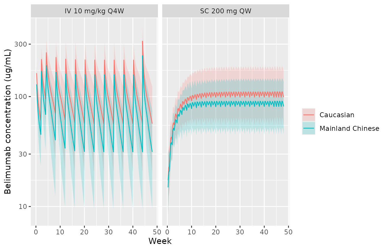
Simulated belimumab concentrations (median and 90% prediction interval) over the first year; compare the IV and SC panels of Wu 2025 Figure S1.
PKNCA: steady-state average concentration
Cavg_ss is computed by PKNCA over the final dosing
interval (days 308-336 for IV, 329-336 for SC), grouped by treatment
arm.
conc_df <- sim |>
  filter(!is.na(Cc)) |>
  select(id, time, Cc, arm)
dose_df <- events |>
  filter(evid == 1) |>
  select(id, time, amt, arm)

conc_obj <- PKNCA::PKNCAconc(conc_df, Cc ~ time | arm + id, concu = "ug/mL", timeu = "day")
dose_obj <- PKNCA::PKNCAdose(dose_df, amt ~ time | arm + id, doseu = "mg")
intervals <- bind_rows(
  data.frame(arm = grep("IV", unique(conc_df$arm), value = TRUE), start = 308, end = 336),
  data.frame(arm = grep("SC", unique(conc_df$arm), value = TRUE), start = 329, end = 336)
) |>
  mutate(cav = TRUE, cmax = TRUE, cmin = TRUE)
nca_res <- PKNCA::pk.nca(PKNCA::PKNCAdata(conc_obj, dose_obj, intervals = intervals))
nca_tbl <- as.data.frame(nca_res$result)
reference <- data.frame(
  arm = c(
    "Caucasian, IV 10 mg/kg Q4W", "Caucasian, SC 200 mg QW",
    "Mainland Chinese, IV 10 mg/kg Q4W", "Mainland Chinese, SC 200 mg QW"
  ),
  cav = c(112.0, 103.1, 70.2, 81.1)
)
cmp <- nlmixr2lib::ncaComparisonTable(
  simulated = filter(nca_tbl, PPTESTCD == "cav"),
  reference = reference,
  by = "arm",
  units = c(cav = "ug/mL")
)
knitr::kable(cmp, caption = "Median Cavg_ss: simulated (PKNCA, 200 per arm) against Wu 2025 Table 4 (5000 per region).")| NCA parameter | arm | Reference | Simulated | % diff |
|---|---|---|---|---|
| Cavg (ug/mL) | Caucasian, IV 10 mg/kg Q4W | 112 | 112 | -0.4% |
| Cavg (ug/mL) | Caucasian, SC 200 mg QW | 103 | 106 | +2.4% |
| Cavg (ug/mL) | Mainland Chinese, IV 10 mg/kg Q4W | 70.2 | 76.5 | +9.0% |
| Cavg (ug/mL) | Mainland Chinese, SC 200 mg QW | 81.1 | 86.7 | +6.9% |
cav_chk <- nca_tbl |>
  filter(PPTESTCD == "cav") |>
  group_by(arm) |>
  summarise(med = median(PPORRES), .groups = "drop") |>
  left_join(reference, by = "arm") |>
  mutate(pct = 100 * (med - cav) / cav)
stopifnot(all(abs(cav_chk$pct) < 15))
cav_ind <- nca_tbl |>
  filter(PPTESTCD == "cav") |>
  left_join(distinct(cohort, id, region, route), by = "id")
ggplot(cav_ind, aes(region, PPORRES, fill = region)) +
  geom_boxplot(outlier.size = 0.5) +
  facet_wrap(~route) +
  labs(x = NULL, y = "Cavg_ss (ug/mL)") +
  theme(legend.position = "none")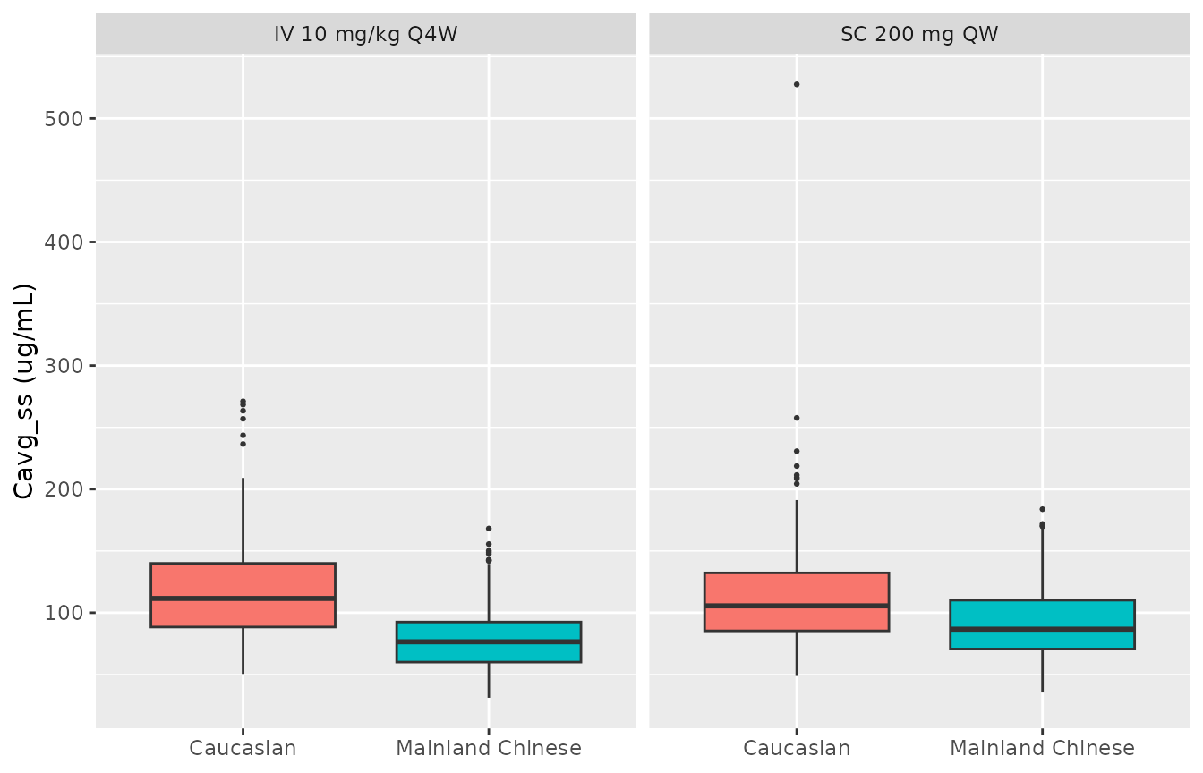
Simulated Cavg_ss by region and regimen; compare the lower panel of Wu 2025 Figure 1.
The Table 4 medians come from 5000 participants per region resampled from the real covariate data; the virtual cohort here is reconstructed from medians and 90% ranges, so agreement within about 10% is what to expect.
E-R: reproducing Table S3
Table S3 tabulates the model-predicted probability of an SRI response
for every combination of race group, SELENA-SLEDAI category and study,
both on placebo (Cavg_ss = 0) and at the maximal treatment
effect (Cavg_ss far above EC50). Solving the packaged E-R
model at those settings reproduces every cell.
solve_er <- function(d) {
  d <- d |>
    mutate(id = row_number(), time = 0, evid = 0L, amt = NA_real_)
  out <- rxode2::rxSolve(rxode2::zeroRe(ui_er), d, returnType = "data.frame")
  out$prob_sri
}

grid <- tidyr::expand_grid(
  race = c("Caucasian or Asian", "Black African ancestry", "Hawaiian or Native American"),
  sledai = c("<10", ">=10"),
  study = c("Studies except BEL112341", "BEL112341"),
  effect = c("Placebo", "Maximal")
) |>
  mutate(
    RACE_BLACK = as.integer(race == "Black African ancestry"),
    RACE_NATIVE_AMERICAN_HAWAIIAN = as.integer(race == "Hawaiian or Native American"),
    SCORE_SLEDAI = ifelse(sledai == ">=10", 12, 6),
    STUDY_BEL112341 = as.integer(study == "BEL112341"),
    CAV = ifelse(effect == "Placebo", 0, 1e8)
  )
grid$sim <- 100 * solve_er(grid)
#> Warning: No omega parameters in the model
#> Warning: multi-subject simulation without without 'omega'

pub_s3 <- tibble::tribble(
  ~effect, ~sledai, ~study, ~`Caucasian or Asian`, ~`Black African ancestry`, ~`Hawaiian or Native American`,
  "Placebo", "<10", "Studies except BEL112341", 31.2, 23.8, 40.3,
  "Placebo", "<10", "BEL112341", 40.5, 31.9, 50.2,
  "Placebo", ">=10", "Studies except BEL112341", 43.6, 34.7, 53.4,
  "Placebo", ">=10", "BEL112341", 53.7, 44.3, 63.2,
  "Maximal", "<10", "Studies except BEL112341", 37.2, 29.0, 46.8,
  "Maximal", "<10", "BEL112341", 47.1, 37.9, 56.9,
  "Maximal", ">=10", "Studies except BEL112341", 62.6, 53.5, 71.3,
  "Maximal", ">=10", "BEL112341", 75.1, 63.3, 78.8
) |>
  pivot_longer(-c(effect, sledai, study), names_to = "race", values_to = "pub")

s3 <- left_join(grid, pub_s3, by = c("race", "sledai", "study", "effect")) |>
  mutate(diff = sim - pub)

s3 |>
  select(effect, sledai, study, race, pub, sim, diff) |>
  mutate(sim = round(sim, 1), diff = round(diff, 2)) |>
  dplyr::rename(
    `Effect` = effect, `SELENA-SLEDAI` = sledai, `Study` = study, `Race` = race,
    `Table S3 Presp (%)` = pub, `Model (%)` = sim, `Difference (points)` = diff
  ) |>
knitr::kable(caption = "Probability of SRI response at Week 52: Wu 2025 Table S3 against the packaged model.")| Effect | SELENA-SLEDAI | Study | Race | Table S3 Presp (%) | Model (%) | Difference (points) |
|---|---|---|---|---|---|---|
| Placebo | <10 | Studies except BEL112341 | Caucasian or Asian | 31.2 | 31.2 | 0.04 |
| Maximal | <10 | Studies except BEL112341 | Caucasian or Asian | 37.2 | 37.2 | 0.04 |
| Placebo | <10 | BEL112341 | Caucasian or Asian | 40.5 | 40.5 | -0.01 |
| Maximal | <10 | BEL112341 | Caucasian or Asian | 47.1 | 47.1 | -0.04 |
| Placebo | >=10 | Studies except BEL112341 | Caucasian or Asian | 43.6 | 43.6 | 0.03 |
| Maximal | >=10 | Studies except BEL112341 | Caucasian or Asian | 62.6 | 62.6 | -0.02 |
| Placebo | >=10 | BEL112341 | Caucasian or Asian | 53.7 | 53.7 | -0.01 |
| Maximal | >=10 | BEL112341 | Caucasian or Asian | 75.1 | 71.5 | -3.63 |
| Placebo | <10 | Studies except BEL112341 | Black African ancestry | 23.8 | 23.8 | -0.01 |
| Maximal | <10 | Studies except BEL112341 | Black African ancestry | 29.0 | 29.0 | -0.03 |
| Placebo | <10 | BEL112341 | Black African ancestry | 31.9 | 31.9 | -0.04 |
| Maximal | <10 | BEL112341 | Black African ancestry | 37.9 | 37.9 | 0.02 |
| Placebo | >=10 | Studies except BEL112341 | Black African ancestry | 34.7 | 34.7 | 0.03 |
| Maximal | >=10 | Studies except BEL112341 | Black African ancestry | 53.5 | 53.5 | -0.03 |
| Placebo | >=10 | BEL112341 | Black African ancestry | 44.3 | 44.3 | 0.05 |
| Maximal | >=10 | BEL112341 | Black African ancestry | 63.3 | 63.3 | -0.05 |
| Placebo | <10 | Studies except BEL112341 | Hawaiian or Native American | 40.3 | 40.3 | -0.05 |
| Maximal | <10 | Studies except BEL112341 | Hawaiian or Native American | 46.8 | 46.8 | 0.01 |
| Placebo | <10 | BEL112341 | Hawaiian or Native American | 50.2 | 50.2 | 0.02 |
| Maximal | <10 | BEL112341 | Hawaiian or Native American | 56.9 | 56.9 | -0.04 |
| Placebo | >=10 | Studies except BEL112341 | Hawaiian or Native American | 53.4 | 53.4 | 0.04 |
| Maximal | >=10 | Studies except BEL112341 | Hawaiian or Native American | 71.3 | 71.3 | -0.04 |
| Placebo | >=10 | BEL112341 | Hawaiian or Native American | 63.2 | 63.2 | 0.03 |
| Maximal | >=10 | BEL112341 | Hawaiian or Native American | 78.8 | 78.8 | -0.01 |
Twenty-three of the 24 cells agree to within rounding (0.05 percentage points). The exception is Caucasian or Asian, SELENA-SLEDAI >= 10, BEL112341, maximal effect: the model gives 71.5% against the printed 75.1%. The same row for the other two race groups (63.3% and 78.8%) follows the Table 3 expression to within rounding, and both differ from the Caucasian or Asian cell only by the race shift on the placebo effect, so the printed 75.1% cannot be produced by the Table 3 estimates. It is taken to be a transcription slip in the supplement.
E-R: exposure-response curve
cav_grid <- seq(0, 250, by = 1)
curve <- tidyr::expand_grid(CAV = cav_grid, SCORE_SLEDAI = c(6, 12)) |>
  mutate(STUDY_BEL112341 = 0L, RACE_BLACK = 0L, RACE_NATIVE_AMERICAN_HAWAIIAN = 0L)
curve$prob <- solve_er(curve)
#> Warning: No omega parameters in the model
#> Warning: multi-subject simulation without without 'omega'
curve |>
  mutate(sledai = ifelse(SCORE_SLEDAI >= 10, "SELENA-SLEDAI >= 10", "SELENA-SLEDAI < 10")) |>
  ggplot(aes(CAV, 100 * prob, colour = sledai)) +
  geom_line() +
  geom_vline(xintercept = exp(ini_er[["lec50"]]), linetype = "dashed") +
  labs(x = "Cavg_ss (ug/mL)", y = "SRI response at Week 52 (%)", colour = NULL)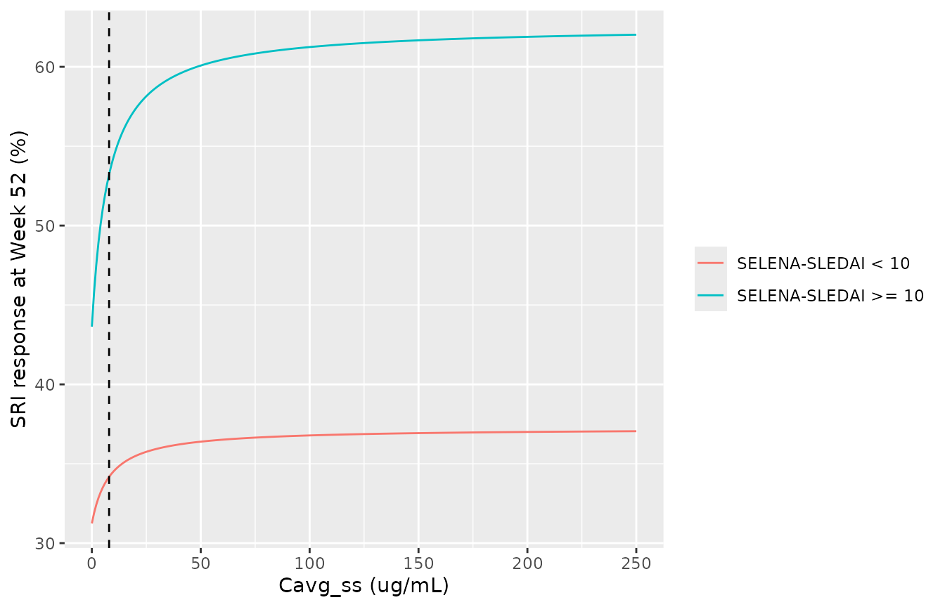
SRI response probability against Cavg_ss for a Caucasian or Asian patient outside study BEL112341; compare the upper panel of Wu 2025 Figure 1 (which averages over the observed covariate mix).
Two numbers in the Results follow from EC50 alone and are reproduced
here: EC90 = 9 x EC50, and the fraction of the maximal effect reached at
the 2.5th percentile of therapeutic Cavg_ss (50.0
ug/mL).
Linking the two models: regional efficacy at the simulated exposures
Wu 2025 concludes that the lower Mainland Chinese exposure changes
the SRI response by less than 2 percentage points (Table 5). Feeding
each virtual participant’s PKNCA Cavg_ss into the E-R model
for a fixed patient profile (Caucasian or Asian, SELENA-SLEDAI >= 10,
outside BEL112341) reproduces the plateau behaviour.
linked <- cav_ind |>
  transmute(
    region, route,
    CAV = PPORRES, SCORE_SLEDAI = 12, STUDY_BEL112341 = 0L,
    RACE_BLACK = 0L, RACE_NATIVE_AMERICAN_HAWAIIAN = 0L
  )
linked$prob <- 100 * solve_er(linked)
#> Warning: No omega parameters in the model
#> Warning: multi-subject simulation without without 'omega'
linked_sum <- linked |>
  group_by(route, region) |>
  summarise(`Median SRI response (%)` = round(median(prob), 2), .groups = "drop")
knitr::kable(linked_sum, caption = "Median predicted SRI response at the simulated Cavg_ss.")| route | region | Median SRI response (%) |
|---|---|---|
| IV 10 mg/kg Q4W | Caucasian | 61.37 |
| IV 10 mg/kg Q4W | Mainland Chinese | 60.87 |
| SC 200 mg QW | Caucasian | 61.31 |
| SC 200 mg QW | Mainland Chinese | 61.05 |
Assumptions and deviations
-
Age constant on Vc. Table S2 prints the Age row
(theta16 in AGE/(AGE + theta16)) as 0.311 with RSE 11.6% and 95% CI
2.08-3.30. The CI excludes 0.311; its midpoint is 2.69 and its
half-width / 1.96 is 0.311, and 0.311 / 2.69 = 11.6% is the printed RSE.
The printed value is therefore the standard error, and the maintainers
use 2.69. The predecessor model (
Zhou_2021_belimumab, same group and same functional form) estimated 1.58. The choice affects Vc only, and only in children:
ages <- c(6, 10, 14, 18, 40)
tibble::tibble(
  `Age (years)` = ages,
  `Vc factor, theta16 = 2.69 (packaged)` = round(ages / (ages + 2.69), 3),
  `Vc factor, theta16 = 0.311 (as printed)` = round(ages / (ages + 0.311), 3)
) |>
knitr::kable()| Age (years) | Vc factor, theta16 = 2.69 (packaged) | Vc factor, theta16 = 0.311 (as printed) |
|---|---|---|
| 6 | 0.690 | 0.951 |
| 10 | 0.788 | 0.970 |
| 14 | 0.839 | 0.978 |
| 18 | 0.870 | 0.983 |
| 40 | 0.937 | 0.992 |
-
Albumin on Vc. The Table S2 footnote equation for
V2 includes (ALB/41)^theta12, but the table lists albumin only under CL,
and the Results name albumin and IgG as covariates of CL. The table is
followed. Had the equation been literal, Vc would scale by
(ALB/41)^-1.11: x 1.31 at 32 g/L and x 0.87 at 46 g/L;
Cavg_ss, and so the E-R link, would not change. - IgG exponent label. The CL equation prints the IgG exponent as theta18; no theta18 exists and the IgG row is theta13 = 0.313, which is used.
-
Residual-error eta. The residual equation prints
the multiplier as exp(eta5), which is the Vp eta. The table and footnote
f attach a separate variance (omega8^2 = 0.272) to the residual error,
so it is encoded as its own
etaRUVscaling both residual SDs. Theta8 and theta9 are standard deviations (the “Uppsala approach” fixes SIGMA to 1). - Albumin unit. The Results give the reference albumin as “41.0 g dL-1”; Table S1 reports albumin in g/L with a median of 41.0, so the reference is 41 g/L.
-
Cavg_ss unit in Table 2. Table 2 prints
Cavg_ssin ng/mL; the text, Table 3 (EC50 in ug/mL) and Table 4 use ug/mL, which the PK model reproduces. - Omitted random effects. The IIV variances on F (omega3) and Q (omega4) are 0 in the source and are not included.
- Table S3 cell. One of the 24 Table S3 probabilities (Caucasian or Asian, SELENA-SLEDAI >= 10, BEL112341, maximal effect: 75.1% printed, 71.5% from Table 3) does not follow the Table 3 expression; see the Table S3 section.
-
E-R residual. The E-R model was fitted with a
Bernoulli likelihood. The file carries a placeholder additive residual
of 0.001 on
prob_sriso that rxode2 has an error model; it is not a published quantity.SCORE_SLEDAIenters only through the indicator SCORE_SLEDAI >= 10. - Virtual cohorts. The PK cohorts are drawn as log-normal distributions matching the Table 4 medians and 90% ranges, with fat-free mass set proportional to body weight (Table 4 median ratio) and adult ages from Table 2. Individual covariate data were not available. Healthy volunteers and children are not simulated.
-
Race coding. The E-R race groups map to
RACE_BLACK(Black African ancestry) and the compositeRACE_NATIVE_AMERICAN_HAWAIIAN(Hawaiian or Native American, fitted as one level); Asian and Caucasian patients are the reference.