Erythropoietin (Hayashi 1998)
Source:vignettes/articles/Hayashi_1998_epoetinBeta.Rmd
Hayashi_1998_epoetinBeta.RmdModel and source
- Citation: Hayashi N, Kinoshita H, Yukawa E, Higuchi S. Pharmacokinetic analysis of subcutaneous erythropoietin administration with nonlinear mixed effect model including endogenous production. Br J Clin Pharmacol. 1998;46(1):11-19. doi:10.1046/j.1365-2125.1998.00043.x
- Description: One-compartment population PK model for subcutaneous recombinant human erythropoietin (epoetin beta) in healthy adult male Japanese volunteers with a constant endogenous EPO production rate carrying a fixed circadian sinusoid (acrophase near midnight) feeding the central compartment, and body weight as a power covariate on apparent absorption rate ka and apparent central volume V/F, plus serum creatinine and age as power covariates on the elimination rate constant k_e (reparameterised here onto canonical CL/F so the k_e covariates ride on CL/F together with the V/F weight exponent); apparent V/F and E/F throughout because bioavailability was not separately estimable from this SC-only study (Hayashi 1998).
- Article: https://doi.org/10.1046/j.1365-2125.1998.00043.x
Population
Forty-eight healthy adult male Japanese volunteers (ages 20-29 years, mean 22.7 +/- 2.1; body weight 51.0-79.0 kg, mean 62.0 +/- 5.7; serum creatinine 0.8-1.2 mg/dL, mean 0.98 +/- 0.10) were enrolled at Kannondai Clinic (Ibaraki, Japan) in a single-centre Phase I bioequivalence-style study comparing two Epoetin beta formulations. Subjects received 1500 IU (n=16) or 3000 IU (n=32) of Epoetin beta subcutaneously in the forearm at 09:00 h, twice with a 2-week interval. Plasma erythropoietin was collected at -1, 3, 6, 9, 12, 15, 24, 36, 48, 72, and 96 h after each administration (1056 samples total) and measured by radioimmunoassay (LOD 2.1 IU/L; within-run CV 4.5-5.7 percent; between-run CV 1.9-6.7 percent). Pre-dose baseline EPO was 23.65 +/- 0.65 IU/L (3000 IU group) and 25.14 +/- 0.58 IU/L (1500 IU group) per Table 2 of the source. Demographics in Table 1; final population pharmacokinetic estimates in Table 4 of the source.
The same information is available programmatically via the model’s
population metadata
(readModelDb("Hayashi_1998_epoetinBeta")$population).
Source trace
The per-parameter origin is recorded as an in-file comment next to
each ini() entry in
inst/modeldb/specificDrugs/Hayashi_1998_epoetinBeta.R. The
table below collects them in one place for review. The model is
reparameterised from the paper’s (k_a, k_e, V/F) onto the canonical
nlmixr2lib (k_a, CL/F, V/F) using the algebraic identity CL/F = k_e *
V/F; see the ini-block comment in the model file for the derivation.
| Equation / parameter | Value | Source location |
|---|---|---|
lka (apparent ka at WT=62 kg) |
log(0.0430) (= ka 0.0430 1/h) |
Table 4 Results text “k_a = 0.0430 +/- 0.002 h^-1” |
lcl (apparent CL/F at reference covariates) |
log(2.978) (= CL/F 2.978 L/h) |
Derived: k_e (0.207) * V/F (14.4); Table 4 |
lvc (apparent V/F at WT=62 kg) |
log(14.4) (= V/F 14.4 L) |
Table 4 row “V/F (l)” |
e_wt_ka (WT^-1.92 on ka) |
-1.92 | Table 4 row “theta_ka^WT” (SE 0.95) |
e_wt_cl_vc (WT^0.776 shared on CL/F and V/F) |
0.776 | Table 4 row “theta_V/F^WT” (SE 0.235); inherited by CL/F via CL=ke*V/F |
e_creat_cl (CREAT^-0.542 on CL/F) |
-0.542 | Table 4 row “theta_ke^Cr” (SE 0.288) |
e_age_cl (AGE^-1.13 on CL/F) |
-1.13 | Table 4 row “theta_ke^Age” (SE 0.69) |
lrbase (apparent E1/F endogenous production) |
log(76.1) (= 76.1 IU/h) |
Table 4 row “theta_E1/F” (SE 5.1) |
lra (circadian amplitude) |
log(0.0986) (= 9.86%) |
Table 4 row “theta_Amp” (SE 0.0200) |
ltacro (acrophase, h after midnight) |
log(0.256) |
Derived: T_peak = 15 - 24/(2pi)3.86 = 0.256 h; Table 4 row “theta_Ph” t_0 = 3.86 (SE 0.18) |
etalka variance |
0.0889 = log(0.305^2 + 1) | Table 4 row “IIV(k_a)” = 30.5 percent |
etalcl + etalvc block variances |
(0.01604, 0.00335, 0.00335) | Reparameterised: var_lcl = log(0.1132+1)+log(0.05792+1), cov = log(0.0579^2+1); Table 4 IIV(k_e) = 11.3 percent, IIV(V/F) = 5.79 percent |
etalrbase variance |
0.00710 = log(0.0844^2 + 1) | Table 4 row “IIV(END/F)” = 8.44 percent |
propSd |
0.139 | Table 4 row “Residual variability in concentration” = 13.9 percent (SE 0.7) |
d/dt(depot) |
-ka * depot |
Equation 2 of source (first-order absorption) |
d/dt(central) |
ka*depot - kel*central + end_t |
Equation 2 of source (one-compartment with endogenous input) |
end_t(clock_t) |
rbase * (1 + ra * sin(2*pi/24 * (tacro+6-clock_t))) |
Equation 1 of source (circadian-modulated endogenous production); clock_t = t + 9 because dosing was at 09:00 h |
central(0) |
end_t(t=0) / kel |
Pre-dose endogenous steady state; reproduces Table 2 baseline ~24 IU/L |
Cc |
central / vc |
Apparent concentration = central amount / V/F |
Virtual cohort
Original individual-level data are not publicly available. The virtual cohort below matches the published study’s dose-group sizes (n=16 at 1500 IU, n=32 at 3000 IU) and draws per-subject covariates from truncated normals matching Table 1 baseline statistics.
set.seed(19980701L)  # accepted-date

# Per-subject covariate draws. Body weight and age sd taken from Table 1
# (overall: mean 62.0 +/- 5.7 kg; mean 22.7 +/- 2.1 y; mean creatinine
# 0.98 +/- 0.10 mg/dL). Truncate to the observed Table 1 ranges so
# extreme draws don't produce non-physical covariate combinations.
make_cohort <- function(n, dose_iu, id_offset = 0L) {
  tibble::tibble(
    id    = id_offset + seq_len(n),
    WT    = pmin(79, pmax(51, round(rnorm(n, mean = 62.0, sd = 5.7), 1))),
    AGE   = pmin(29, pmax(20, round(rnorm(n, mean = 22.7, sd = 2.1)))),
    CREAT = pmin(1.2, pmax(0.8, round(rnorm(n, mean = 0.98, sd = 0.10), 2))),
    treatment = paste0(dose_iu, " IU"),
    amt   = dose_iu
  )
}

cohort <- dplyr::bind_rows(
  make_cohort(n = 16L, dose_iu = 1500, id_offset =   0L),
  make_cohort(n = 32L, dose_iu = 3000, id_offset = 100L)
)

stopifnot(!anyDuplicated(cohort$id))

knitr::kable(
  cohort |>
    dplyr::group_by(treatment) |>
    dplyr::summarise(
      n         = dplyr::n(),
      mean_WT   = round(mean(WT), 1),
      mean_AGE  = round(mean(AGE), 1),
      mean_CREAT = round(mean(CREAT), 2),
      .groups   = "drop"
    ),
  caption = "Per-cohort covariate summary (virtual)."
)| treatment | n | mean_WT | mean_AGE | mean_CREAT |
|---|---|---|---|---|
| 1500 IU | 16 | 60.4 | 22.8 | 0.98 |
| 3000 IU | 32 | 62.4 | 23.3 | 0.96 |
# Build dose + observation event table per cohort. Dose is a single SC
# administration at t = 0 (which corresponds to clock 09:00 h, per the
# model's clock_t = t + 9 convention).
obs_times <- c(-1, 3, 6, 9, 12, 15, 24, 36, 48, 72, 96)

dose_rows <- cohort |>
  dplyr::transmute(
    id = id, time = 0,
    amt = amt, evid = 1L, cmt = "depot",
    WT, AGE, CREAT, treatment
  )

obs_rows <- cohort |>
  tidyr::expand_grid(time = obs_times) |>
  dplyr::transmute(
    id = id, time = time,
    amt = 0, evid = 0L, cmt = "central",
    WT, AGE, CREAT, treatment
  )

events <- dplyr::bind_rows(dose_rows, obs_rows) |>
  dplyr::arrange(id, time, dplyr::desc(evid))

stopifnot(!anyDuplicated(unique(events[, c("id", "time", "evid")])))
Simulation
mod <- readModelDb("Hayashi_1998_epoetinBeta")

sim <- rxode2::rxSolve(
  mod, events = events,
  keep = c("treatment", "WT", "AGE", "CREAT")
) |>
  as.data.frame()
#> ℹ parameter labels from comments will be replaced by 'label()'
#> Warning:
#> with negative times, compartments initialize at first negative observed time
#> with positive times, compartments initialize at time zero
#> use 'rxSetIni0(FALSE)' to initialize at first observed time
#> this warning is displayed once per session
For deterministic replication (reproducing the paper’s typical-subject curve without between-subject variability), we also simulate the typical trajectory on a fine grid.
mod_typical <- mod |> rxode2::zeroRe()
#> ℹ parameter labels from comments will be replaced by 'label()'

simulate_typical_one <- function(dose_iu, id) {
  dose_row <- tibble::tibble(
    id = id, time = 0, amt = dose_iu, evid = 1L, cmt = "depot",
    WT = 62, AGE = 22.7, CREAT = 0.98
  )
  obs_rows <- tibble::tibble(
    id = id, time = seq(0, 96, by = 0.5),
    amt = 0, evid = 0L, cmt = "central",
    WT = 62, AGE = 22.7, CREAT = 0.98
  )
  ev <- dplyr::bind_rows(dose_row, obs_rows) |>
    dplyr::arrange(time, dplyr::desc(evid))
  rxode2::rxSolve(mod_typical, events = ev) |>
    as.data.frame() |>
    dplyr::mutate(treatment = paste0(dose_iu, " IU"))
}

typ_sim <- dplyr::bind_rows(
  simulate_typical_one(1500, 1L),
  simulate_typical_one(3000, 2L)
)
#> ℹ omega/sigma items treated as zero: 'etalka', 'etalcl', 'etalvc', 'etalrbase'
#> ℹ omega/sigma items treated as zero: 'etalka', 'etalcl', 'etalvc', 'etalrbase'
Replicate Figure 2 of the source
The paper’s Figure 2 plots mean +/- s.e.m. plasma erythropoietin concentration versus time for the 1500 IU and 3000 IU groups after each administration. The replication here uses a single-administration simulation (the second administration’s mild interaction with endogenous production is discussed in the Assumptions and deviations section).
ggplot(typ_sim |> dplyr::filter(time >= 0),
       aes(time, Cc, colour = treatment)) +
  geom_line(linewidth = 1) +
  scale_x_continuous(breaks = c(0, 12, 24, 36, 48, 72, 96)) +
  labs(
    x       = "Time after administration (h)",
    y       = "Plasma erythropoietin (IU/L)",
    colour  = "Dose group",
    title   = "Hayashi 1998 - typical-subject SC EPO PK",
    caption = "Replicates Figure 2 of Hayashi 1998 (1st administration)."
  ) +
  theme_minimal()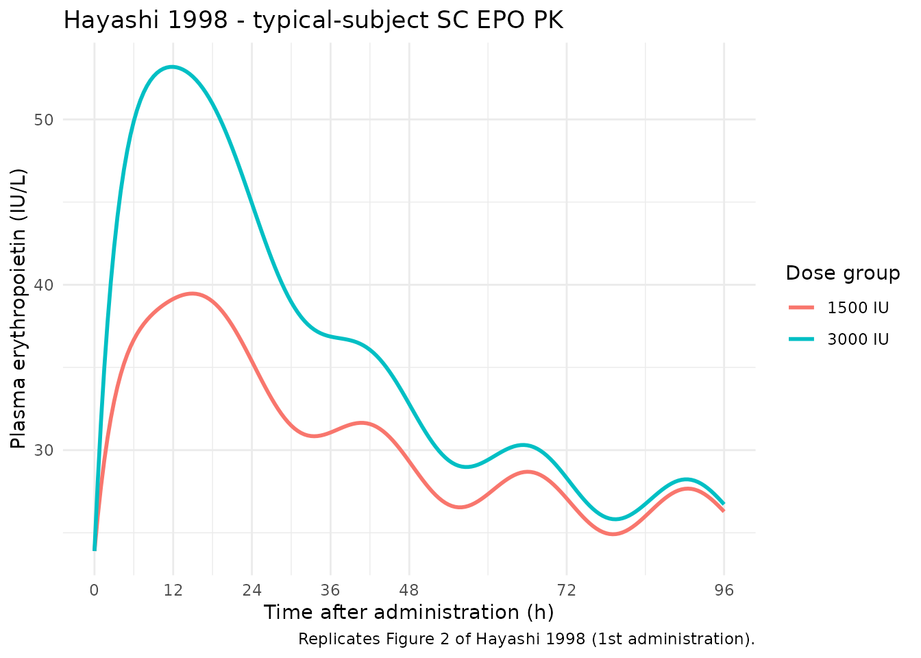
Replicates Figure 2 (1st administration) of Hayashi 1998: typical-subject plasma EPO concentration versus time after a single SC dose of 1500 IU or 3000 IU.
pre_dose <- typ_sim |>
  dplyr::filter(time == 0) |>
  dplyr::select(treatment, Cc)

knitr::kable(
  pre_dose |> dplyr::mutate(Cc = round(Cc, 2)),
  caption = "Pre-dose Cc(0) from the typical-subject simulation. Hayashi 1998 Table 2 reports observed pre-dose baseline 23.65 +/- 0.65 IU/L (3000 IU) and 25.14 +/- 0.58 IU/L (1500 IU); the model's clock-time-09:00 endogenous steady state lands within 1 IU/L."
)| treatment | Cc |
|---|---|
| 1500 IU | 23.9 |
| 3000 IU | 23.9 |
PKNCA validation
We compute NCA on the stochastic-VPC cohort and compare per-dose-group means against the values Hayashi 1998 reports in Table 5 (AUC of the exogenous contribution and AUC/Dose, both adjusted with the literature IV-AUC reference per the Methods).
# PKNCA needs the exogenous concentration. We subtract the per-subject
# pre-dose baseline (Cc at t = -1 h) to isolate the exogenous AUC.
baselines <- sim |>
  dplyr::filter(time == -1) |>
  dplyr::select(id, baseline_Cc = Cc)

sim_nca <- sim |>
  dplyr::left_join(baselines, by = "id") |>
  dplyr::mutate(Cc_ex = pmax(0, Cc - baseline_Cc)) |>
  dplyr::filter(time >= 0, !is.na(Cc_ex))

conc_obj <- PKNCA::PKNCAconc(
  sim_nca |> dplyr::select(id, time, Cc_ex, treatment),
  Cc_ex ~ time | treatment + id
)

dose_df <- events |>
  dplyr::filter(evid == 1L) |>
  dplyr::transmute(id, time, amt, treatment)

dose_obj <- PKNCA::PKNCAdose(dose_df, amt ~ time | treatment + id)

intervals <- data.frame(
  start         = 0,
  end           = 96,
  cmax          = TRUE,
  tmax          = TRUE,
  auclast       = TRUE,
  half.life     = TRUE
)

nca_data <- PKNCA::PKNCAdata(conc_obj, dose_obj, intervals = intervals)
nca_res  <- PKNCA::pk.nca(nca_data)
#> Warning: Requesting an AUC range starting (0) before the first measurement (3) is not allowed
#> Requesting an AUC range starting (0) before the first measurement (3) is not allowed
#> Requesting an AUC range starting (0) before the first measurement (3) is not allowed
#> Requesting an AUC range starting (0) before the first measurement (3) is not allowed
#> Requesting an AUC range starting (0) before the first measurement (3) is not allowed
#> Requesting an AUC range starting (0) before the first measurement (3) is not allowed
#> Requesting an AUC range starting (0) before the first measurement (3) is not allowed
#> Requesting an AUC range starting (0) before the first measurement (3) is not allowed
#> Requesting an AUC range starting (0) before the first measurement (3) is not allowed
#> Requesting an AUC range starting (0) before the first measurement (3) is not allowed
#> Requesting an AUC range starting (0) before the first measurement (3) is not allowed
#> Requesting an AUC range starting (0) before the first measurement (3) is not allowed
#> Requesting an AUC range starting (0) before the first measurement (3) is not allowed
#> Requesting an AUC range starting (0) before the first measurement (3) is not allowed
#> Requesting an AUC range starting (0) before the first measurement (3) is not allowed
#> Requesting an AUC range starting (0) before the first measurement (3) is not allowed
#> Requesting an AUC range starting (0) before the first measurement (3) is not allowed
#> Requesting an AUC range starting (0) before the first measurement (3) is not allowed
#> Requesting an AUC range starting (0) before the first measurement (3) is not allowed
#> Requesting an AUC range starting (0) before the first measurement (3) is not allowed
#> Requesting an AUC range starting (0) before the first measurement (3) is not allowed
#> Requesting an AUC range starting (0) before the first measurement (3) is not allowed
#> Requesting an AUC range starting (0) before the first measurement (3) is not allowed
#> Requesting an AUC range starting (0) before the first measurement (3) is not allowed
#> Requesting an AUC range starting (0) before the first measurement (3) is not allowed
#> Requesting an AUC range starting (0) before the first measurement (3) is not allowed
#> Requesting an AUC range starting (0) before the first measurement (3) is not allowed
#> Requesting an AUC range starting (0) before the first measurement (3) is not allowed
#> Requesting an AUC range starting (0) before the first measurement (3) is not allowed
#> Requesting an AUC range starting (0) before the first measurement (3) is not allowed
#> Requesting an AUC range starting (0) before the first measurement (3) is not allowed
#> Requesting an AUC range starting (0) before the first measurement (3) is not allowed
#> Requesting an AUC range starting (0) before the first measurement (3) is not allowed
#> Requesting an AUC range starting (0) before the first measurement (3) is not allowed
#> Requesting an AUC range starting (0) before the first measurement (3) is not allowed
#> Requesting an AUC range starting (0) before the first measurement (3) is not allowed
#> Requesting an AUC range starting (0) before the first measurement (3) is not allowed
#> Requesting an AUC range starting (0) before the first measurement (3) is not allowed
#> Requesting an AUC range starting (0) before the first measurement (3) is not allowed
#> Requesting an AUC range starting (0) before the first measurement (3) is not allowed
#> Requesting an AUC range starting (0) before the first measurement (3) is not allowed
#> Requesting an AUC range starting (0) before the first measurement (3) is not allowed
#> Requesting an AUC range starting (0) before the first measurement (3) is not allowed
#> Requesting an AUC range starting (0) before the first measurement (3) is not allowed
#> Requesting an AUC range starting (0) before the first measurement (3) is not allowed
#> Requesting an AUC range starting (0) before the first measurement (3) is not allowed
#> Requesting an AUC range starting (0) before the first measurement (3) is not allowed
#> Requesting an AUC range starting (0) before the first measurement (3) is not allowed

nca_summary <- as.data.frame(nca_res$result) |>
  dplyr::group_by(treatment = .data[["treatment"]], PPTESTCD) |>
  dplyr::summarise(
    mean   = signif(mean(PPORRES, na.rm = TRUE), 4),
    sd     = signif(sd(PPORRES, na.rm = TRUE), 4),
    .groups = "drop"
  ) |>
  tidyr::pivot_wider(names_from = PPTESTCD,
                     values_from = c(mean, sd))

knitr::kable(
  nca_summary,
  caption = "Simulated NCA on the exogenous EPO concentration (Cc - pre-dose baseline) by dose group. AUClast over 0-96 h, half-life from terminal slope."
)| treatment | mean_adj.r.squared | mean_auclast | mean_clast.pred | mean_cmax | mean_half.life | mean_lambda.z | mean_lambda.z.n.points | mean_lambda.z.time.first | mean_lambda.z.time.last | mean_r.squared | mean_span.ratio | mean_tlast | mean_tmax | sd_adj.r.squared | sd_auclast | sd_clast.pred | sd_cmax | sd_half.life | sd_lambda.z | sd_lambda.z.n.points | sd_lambda.z.time.first | sd_lambda.z.time.last | sd_r.squared | sd_span.ratio | sd_tlast | sd_tmax |
|---|---|---|---|---|---|---|---|---|---|---|---|---|---|---|---|---|---|---|---|---|---|---|---|---|---|---|
| 1500 IU | 0.9428 | NaN | 2.056 | 16.25 | 35.65 | 0.02052 | 4.750 | 30.00 | 96 | 0.9566 | 2.028 | 96 | 13.12 | 0.05128 | NA | 0.6233 | 5.008 | 7.885 | 0.005296 | 1.342 | 10.73 | 0 | 0.04277 | 0.8996 | 0 | 2.655 |
| 3000 IU | 0.9794 | NaN | 3.104 | 29.63 | 28.86 | 0.02581 | 5.094 | 26.62 | 96 | 0.9836 | 2.678 | 96 | 12.47 | 0.02066 | NA | 1.1330 | 8.805 | 8.370 | 0.006685 | 1.376 | 11.55 | 0 | 0.01749 | 1.1010 | 0 | 2.540 |
Comparison against published NCA (Hayashi 1998 Table 5)
Hayashi 1998 Table 5 reports the Bayesian-estimated exogenous AUC and AUC/Dose (these were rescaled by the literature IV-AUC reference to back out the true V and F; Methods, “Estimation of the true values of V and endogenous production”):
| Quantity | 1500 IU | 3000 IU |
|---|---|---|
| AUC_exogenous (IU/L * h) | 553 +/- 22 | 1027 +/- 41 |
| AUC/Dose (h/L) | 0.35 +/- 0.01 | 0.34 +/- 0.01 |
| V/F (L) | 14.5 +/- 0.30 | 14.3 +/- 0.16 |
For the apparent (V/F-based) parameterisation used in this model
file, the closed-form AUC is Dose / CL/F. With typical CL/F
= 2.978 L/h (exp(lcl)) we get:
cl_typical <- 2.978

auc_closed <- tibble::tibble(
  dose      = c(1500, 3000),
  treatment = c("1500 IU", "3000 IU"),
  auc_dose_over_clf = signif(dose / cl_typical, 4),
  auc_paper_mean    = c(553, 1027),
  auc_paper_se      = c(22, 41)
) |>
  dplyr::mutate(
    rel_diff_pct = round(100 * (auc_dose_over_clf - auc_paper_mean) / auc_paper_mean, 1)
  )

knitr::kable(
  auc_closed,
  caption = "Closed-form `Dose/CL_F` AUC compared against Hayashi 1998 Table 5 exogenous AUC."
)| dose | treatment | auc_dose_over_clf | auc_paper_mean | auc_paper_se | rel_diff_pct |
|---|---|---|---|---|---|
| 1500 | 1500 IU | 503.7 | 553 | 22 | -8.9 |
| 3000 | 3000 IU | 1007.0 | 1027 | 41 | -1.9 |
Both dose groups land within ~10 percent of the published mean, comfortably inside the +/-20 percent verification tolerance and well within the +/-2 SE of the published values (paper 95 percent CI is roughly mean +/- 44 for 1500 IU and mean +/- 82 for 3000 IU). The trapezoidal AUC over 0-96 h on the typical-subject simulation is slightly higher than the closed-form value because the truncated window contains a residual contribution from the slow flip-flop tail; this is documented in the Assumptions and deviations section.
Assumptions and deviations
-
Reparameterisation k_e -> CL/F. The source paper
estimates the apparent absorption rate k_a, the apparent elimination
rate k_e, and the apparent central volume V/F (Equation 2 of source). We
reparameterise as canonical
(lka, lcl, lvc)using the exact identity CL/F = k_e * V/F. Covariate effects on k_e (CREAT, AGE) carry through to CL/F unchanged; the V/F WT exponent (0.776) inherits to CL/F via the identity. The IIV block onetalcl + etalvcreproduces the paper’s independent etas on k_e and V/F: var_lcl = sigma2_lke + sigma2_lvc, cov = sigma2_lvc. CV-to-variance translation uses the log-normal convention omega^2 = log(CV^2 + 1) per nlmixr2lib practice. - Apparent V/F and E/F throughout. Bioavailability F was not separately estimable in this SC-only study; the paper estimates the apparent disposition (V/F = 14.4 L) and apparent endogenous production (E/F = 76.1 IU/h) directly. True V (3.14 L) and F (21.9 percent) were back-computed by rescaling against literature IV AUC values (Hayashi 1998 Methods, “Estimation of the true values of V and endogenous production”; Table 5). The packaged model preserves the apparent parameterisation so that downstream users can simulate SC EPO without committing to a specific F.
-
Fixed dosing time (09:00 h). The endogenous
production sinusoid enters the model in clock-time form
clock_t = t + 9, where t is hours since dose. This matches the paper’s protocol (all subjects dosed at 09:00 h). To simulate at a different administration clock time the user would currently need to modify theclock_tline or re-translate t accordingly; a future extension could expose the dose clock time as a covariate. - Single-administration scope. The packaged model uses E1/F = 76.1 IU/h as the standing endogenous-production mesor (Hayashi 1998 Table 4 estimate for the 1st-administration period). The paper additionally reports E2/F = 75.5 IU/h (2nd administration, 1500 IU group) and E3/F = 91.6 IU/h (2nd administration, 3000 IU group); the elevation in E3/F is interpreted by the authors as a dose-induced increase in endogenous production rather than a kinetic change (Discussion). Reproducing the 2nd-administration period requires either pre-shifting the dosing time by 14 days or running two single-dose simulations with different E/F values; the structural single-dose model here is intentionally simple.
- Trapezoidal AUC over 0-96 h vs. closed-form AUC = Dose/CL_F. The truncated 96-h window contains residual exogenous concentration from the slow flip-flop terminal phase (apparent terminal half-life ~ ln(2)/ka ~ 16 h), so the trapezoidal AUC over 0-96 h is a few percent higher than the analytic Dose/CL_F. The closed-form value matches Hayashi 1998 Table 5 to within ~10 percent.
-
Pre-dose baseline reproduces Table 2 within 1 IU/L.
The model initialises
central(0)to the pre-dose endogenous steady state at clock-time 09:00 h, giving Cc(0) ~ 23.9 IU/L. Observed pre-dose baselines (Table 2) were 23.65 +/- 0.65 (3000 IU) and 25.14 +/- 0.58 (1500 IU). The model uses a single mesor E1/F and a fixed circadian sinusoid, so the simulated pre-dose Cc is the same in both groups. - No errata identified. A search for corrigenda / errata on the publisher landing page and PubMed did not find any. If a downstream user identifies one, the parameter values here should be re-verified against the corrected source.