SAR439459 (Baranda 2024)
Source:vignettes/articles/Baranda_2024_sar439459.Rmd
Baranda_2024_sar439459.RmdModel and source
- Citation: Baranda JC, Robbrecht D, Sullivan R, Doger B, Santoro A, Barve M, Grob J-J, Bechter O, Vieito M, de Miguel MJ, Schadendorf D, Johnson M, Pouzin C, Cantalloube C, Wang R, Lee J, Chen X, Demers B, Amrate A, Abbadessa G, Hodi FS. Safety, pharmacokinetics, pharmacodynamics, and antitumor activity of SAR439459, a TGFbeta inhibitor, as monotherapy and in combination with cemiplimab in patients with advanced solid tumors: Findings from a phase 1/1b study. Clin Transl Sci. 2024;17(6):e13854. doi:10.1111/cts.13854
- Human model: Two-compartment population PK model with linear elimination for SAR439459 (anti-TGF-beta monoclonal antibody) given intravenously as monotherapy or with cemiplimab in adults with advanced solid tumours, with body weight on clearance and sex on central volume (Baranda 2024)
- Mouse model: Preclinical (mouse, MC38 syngeneic colon tumour). Direct Emax inhibition model of intratumoral active TGF-beta driven by the SAR439459 (anti-TGF-beta monoclonal antibody) plasma concentration, with a study-specific baseline and a shared Emax and EC50 (Baranda 2024)
- Article: https://doi.org/10.1111/cts.13854 (open access, PMC11186846)
Baranda 2024 reports the phase 1/1b study of SAR439459 (SAR’459), a human anti-TGF-beta IgG4 monoclonal antibody that neutralises all three TGF-beta isoforms, given intravenously alone or with cemiplimab. Two models from the paper’s supplement are packaged:
-
Baranda_2024_sar439459– the human population PK model (supplement Table S2), fitted to the 52 dose-escalation patients. -
Baranda_2024_sar439459_mouse– the preclinical PK/PD model in MC38 tumour-bearing mice (supplement Table S3 and Eq. 1), a direct Emax inhibition of intratumoral active TGF-beta by the SAR439459 plasma concentration. Its EC50 (about 30 ug/mL) and near-maximal concentration (about 200 ug/mL) were the exposure targets used to pick the 7.5 and 22.5 mg/kg Q3W expansion doses.
The two models are independent fits in different species; the source does not link them, other than by comparing human simulated troughs with the mouse-derived thresholds (supplement Figure S5). That comparison is reproduced at the end of this article.
Population
Human. The popPK data set holds 52 patients with advanced unresectable or metastatic solid tumours from the dose-escalation parts of NCT03192345: Part 1A (n = 28, SAR439459 0.05-15 mg/kg Q2W monotherapy) and Part 1B (n = 24, SAR439459 0.25-15 mg/kg Q2W or 22.5 mg/kg Q3W with cemiplimab 3 mg/kg Q2W or 350 mg Q3W). Median age was 60.5 years (Part 1A, range 25-91) and 63.0 years (Part 1B, range 43-81); 25 of 52 patients (48.1%) were female (Table 1). Cycle 1 was richly sampled (pre-dose to 336 h, plus 504 h for Q3W) and later cycles sparsely. Body weight is not tabulated.
Mouse. Four MC38 syngeneic colon-carcinoma studies, each with an untreated control group: study 1 (single dose, 1 and 25 mg/kg), study 2 (single dose, 10, 25 and 50 mg/kg), study 3 (three doses of 25 mg/kg) and study 4 (single dose, 10, 25 and 50 mg/kg) (supplement Figure S3A legend). Plasma SAR439459 and intratumoral active TGF-beta (pg/mg total protein) were measured in the same animals at several times after dosing. The number of animals is not reported.
The same information is available programmatically via each model’s
population metadata,
e.g. readModelDb("Baranda_2024_sar439459")()$population.
Source trace
| Equation / parameter | Value | Source location |
|---|---|---|
| Human: two-compartment, linear elimination, IV | – | Results, Population pharmacokinetics; supplement p. 4 |
lcl (CL, 70 kg) |
0.141 L/day | Supplement Table S2 |
e_wt_cl (power on WT/70) |
0.994 | Supplement Table S2 ‘+ betaWT’ |
lvc (Vc, male) |
4.06 L | Supplement Table S2 |
e_sexf_vc (log-scale, female) |
-0.321 | Supplement Table S2 ‘+ betaSEX_female’ |
lq (Q) |
0.624 L/day | Supplement Table S2 |
lvp (Vp) |
2.44 L | Supplement Table S2 |
etalcl, etalvc, etalvp
|
0.337^2, 0.224^2, 0.731^2 | Supplement Table S2 omega (%) = 33.7, 22.4, 73.1 |
propSd (human) |
0.195 | Supplement Table S2 sigma prop = 19.5% |
Mouse: tgfb_tumor = E0 - Emax * C / (EC50 + C)
|
– | Supplement Eq. 1 (see Assumptions) |
le0_tgfb_tumor (study 1) |
52.5 pg/mg protein | Supplement Table S3 |
le0_tgfb_tumor_study2 / _study3 /
_study4
|
44.3 / 58.5 / 61.4 pg/mg protein | Supplement Table S3 |
lemax |
31.7 pg/mg protein | Supplement Table S3 |
lec50 |
29.4 ug/mL | Supplement Table S3 |
propSd (mouse) |
0.311 | Supplement Table S3 ‘Proportional error’ = 31.1% |
Human population PK
Virtual cohort
Body weight is not reported for the PK population, so a log-normal weight with median 70 kg and 20% CV (truncated to 40-130 kg) is assumed; 48.1% of virtual patients are female (Table 1, Parts 1A and 1B). Supplement Figure S5 simulated 200 patients per regimen, which this article matches.
mod_h <- readModelDb("Baranda_2024_sar439459")

n_per_arm <- 200
set.seed(20240611)
rxode2::rxSetSeed(20240611)

cohort <- tibble(
  id_base = seq_len(n_per_arm),
  WT = pmin(pmax(70 * exp(rnorm(n_per_arm, 0, 0.198)), 40), 130),
  SEXF = rbinom(n_per_arm, 1, 0.481)
)

regimens <- tibble(regimen = c("7.5 mg/kg Q3W", "22.5 mg/kg Q3W"), mgkg = c(7.5, 22.5))
dose_days <- seq(0, 189, by = 21)
obs_days <- sort(unique(c(
  seq(0, 210, by = 0.5),
  dose_days + 1 / 24,
  dose_days + 21 - 1e-3
)))

subjects <- tidyr::crossing(regimens, cohort) |>
  mutate(id = row_number(), amt = mgkg * WT)

dose_rows <- subjects |>
  tidyr::crossing(time = dose_days) |>
  mutate(evid = 1L, cmt = "central", dur = 1 / 24)
obs_rows <- subjects |>
  tidyr::crossing(time = obs_days) |>
  mutate(evid = 0L, cmt = "central", amt = 0, dur = 0)

events_h <- bind_rows(dose_rows, obs_rows) |>
  arrange(id, time, desc(evid)) |>
  select(id, time, evid, cmt, amt, dur, WT, SEXF, regimen, mgkg)

sim_h <- rxode2::rxSolve(mod_h, events_h, keep = c("regimen", "mgkg")) |>
  as.data.frame()
#> ℹ parameter labels from comments will be replaced by 'label()'
Replicates Figure S5 (5th, median and 95th percentiles)
pct_h <- sim_h |>
  group_by(regimen, time) |>
  summarise(
    p05 = quantile(Cc, 0.05),
    p50 = median(Cc),
    p95 = quantile(Cc, 0.95),
    .groups = "drop"
  ) |>
  mutate(regimen = factor(regimen, levels = regimens$regimen))

ggplot(pct_h, aes(time)) +
  geom_ribbon(aes(ymin = p05, ymax = p95), fill = "grey80") +
  geom_line(aes(y = p50)) +
  geom_hline(yintercept = c(30, 200), linetype = "dashed") +
  facet_wrap(~regimen, scales = "free_y") +
  scale_x_continuous(breaks = seq(0, 210, by = 21)) +
  labs(
    x = "Time (days)", y = "SAR439459 concentration (ug/mL)",
    caption = "Replicates supplement Figure S5 of Baranda 2024. Dashed lines: 30 and 200 ug/mL."
  )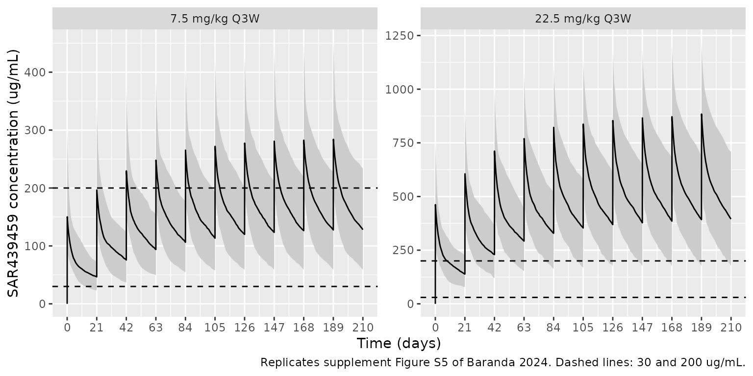
The figure’s medians were digitised by the maintainers from supplement Figure S5 at the end of the first infusion (cycle-1 peak), at day 21 (cycle-1 trough), at the last peak (day 189) and at day 210 (trough after the tenth dose).
at_time <- function(d, t) {
  d |>
    group_by(regimen) |>
    filter(abs(time - t) == min(abs(time - t))) |>
    summarise(p05 = quantile(Cc, 0.05), p50 = median(Cc), .groups = "drop")
}
digitised <- tribble(
  ~regimen, ~landmark, ~t, ~published_median,
  "7.5 mg/kg Q3W", "Cycle-1 peak", 1 / 24, 135,
  "7.5 mg/kg Q3W", "Day-21 trough", 21 - 1e-3, 48,
  "7.5 mg/kg Q3W", "Day-189 peak", 189 + 1 / 24, 300,
  "7.5 mg/kg Q3W", "Day-210 trough", 210, 150,
  "22.5 mg/kg Q3W", "Cycle-1 peak", 1 / 24, 440,
  "22.5 mg/kg Q3W", "Day-21 trough", 21 - 1e-3, 150,
  "22.5 mg/kg Q3W", "Day-189 peak", 189 + 1 / 24, 910,
  "22.5 mg/kg Q3W", "Day-210 trough", 210, 435
)
median_at <- function(reg, t) {
  d <- sim_h[sim_h$regimen == reg, ]
  median(d$Cc[abs(d$time - t) == min(abs(d$time - t))])
}
cmp_s5 <- digitised |>
  mutate(
    simulated_median = mapply(median_at, regimen, t),
    ratio = simulated_median / published_median
  )

cmp_s5 |>
  mutate(across(c(simulated_median, ratio), \(x) signif(x, 3))) |>
  select(-t) |>
  dplyr::rename(
    Regimen = regimen,
    Landmark = landmark,
    "Figure S5 median (ug/mL)" = published_median,
    "Simulated median (ug/mL)" = simulated_median,
    "Simulated / published" = ratio
  ) |>
knitr::kable()| Regimen | Landmark | Figure S5 median (ug/mL) | Simulated median (ug/mL) | Simulated / published |
|---|---|---|---|---|
| 7.5 mg/kg Q3W | Cycle-1 peak | 135 | 150.0 | 1.110 |
| 7.5 mg/kg Q3W | Day-21 trough | 48 | 46.6 | 0.971 |
| 7.5 mg/kg Q3W | Day-189 peak | 300 | 284.0 | 0.947 |
| 7.5 mg/kg Q3W | Day-210 trough | 150 | 128.0 | 0.854 |
| 22.5 mg/kg Q3W | Cycle-1 peak | 440 | 462.0 | 1.050 |
| 22.5 mg/kg Q3W | Day-21 trough | 150 | 139.0 | 0.924 |
| 22.5 mg/kg Q3W | Day-189 peak | 910 | 884.0 | 0.972 |
| 22.5 mg/kg Q3W | Day-210 trough | 435 | 395.0 | 0.909 |
stopifnot(
  # A mis-transcribed CL, Vc, dose or unit shifts every landmark by tens of
  # percent; the digitising error and the assumed weight distribution do not.
  abs(median(log(cmp_s5$ratio))) < log(1.15),
  all(cmp_s5$ratio > 0.75 & cmp_s5$ratio < 1.33)
)
The paper states that 22.5 mg/kg Q3W gives troughs at or above 200 ug/mL and 7.5 mg/kg Q3W gives troughs at or above 30 ug/mL (Results; Figure S5 shows these thresholds against the 5th percentile at steady state and in cycle 1, respectively).
trough_p05 <- bind_rows(
  at_time(sim_h, 21 - 1e-3) |> mutate(when = "Day 21 (cycle 1)"),
  at_time(sim_h, 210) |> mutate(when = "Day 210 (after 10 doses)")
)
trough_p05 |>
  mutate(across(c(p05, p50), \(x) signif(x, 3))) |>
  select(when, regimen, p50, p05) |>
  dplyr::rename(
    Regimen = regimen, Trough = when,
    "5th percentile (ug/mL)" = p05, "Median (ug/mL)" = p50
  ) |>
knitr::kable()| Trough | Regimen | Median (ug/mL) | 5th percentile (ug/mL) |
|---|---|---|---|
| Day 21 (cycle 1) | 22.5 mg/kg Q3W | 139.0 | 78.2 |
| Day 21 (cycle 1) | 7.5 mg/kg Q3W | 46.6 | 23.1 |
| Day 210 (after 10 doses) | 22.5 mg/kg Q3W | 395.0 | 177.0 |
| Day 210 (after 10 doses) | 7.5 mg/kg Q3W | 128.0 | 58.9 |
The simulated 5th percentiles sit a little below these statements (and below the 5th-percentile lines of Figure S5, which read about 28 ug/mL at day 21 for 7.5 mg/kg and about 190 ug/mL at day 210 for 22.5 mg/kg). The lower tail depends on the assumed weight distribution and on the large Vp variability (omega 73.1%), neither of which can be matched exactly from the reported information; the medians, which carry the structural parameters, agree.
PKNCA: cycle-1 exposure
The paper reports no NCA table; cycle-1 NCA is shown for reference and to confirm dose proportionality, which a linear model must give.
conc_c1 <- sim_h |>
  filter(time <= 21, !is.na(Cc)) |>
  select(id, time, Cc, regimen)
dose_c1 <- events_h |>
  filter(evid == 1, time == 0) |>
  select(id, time, amt, regimen)

conc_obj <- PKNCA::PKNCAconc(conc_c1, Cc ~ time | regimen + id)
dose_obj <- PKNCA::PKNCAdose(dose_c1, amt ~ time | regimen + id)
intervals <- data.frame(start = 0, end = 21 - 1e-3, cmax = TRUE, auclast = TRUE, clast.obs = TRUE)
nca_res <- PKNCA::pk.nca(PKNCA::PKNCAdata(conc_obj, dose_obj, intervals = intervals))

nca_tab <- as.data.frame(nca_res$result) |>
  group_by(regimen, PPTESTCD) |>
  summarise(median = median(PPORRES), .groups = "drop") |>
  tidyr::pivot_wider(names_from = PPTESTCD, values_from = median)

nca_tab |>
  mutate(across(-regimen, \(x) signif(x, 3))) |>
  dplyr::rename(
    Regimen = regimen,
    "Cmax (ug/mL)" = cmax,
    "Concentration at day 21 (ug/mL)" = clast.obs,
    "AUC0-21 (day*ug/mL)" = auclast
  ) |>
knitr::kable()| Regimen | AUC0-21 (day*ug/mL) | Concentration at day 21 (ug/mL) | Cmax (ug/mL) |
|---|---|---|---|
| 22.5 mg/kg Q3W | 4400 | 139.0 | 462 |
| 7.5 mg/kg Q3W | 1430 | 46.6 | 150 |
Covariate effects
The paper notes that weight and sex change exposure by less than 30% at the covariate extremes relative to the median. With the typical-value model:
typ <- tidyr::crossing(WT = c(50, 70, 100), SEXF = c(0, 1)) |>
  mutate(
    cl = 0.141 * (WT / 70)^0.994,
    vc = 4.06 * exp(-0.321 * SEXF)
  )
typ |>
  mutate(across(c(cl, vc), \(x) signif(x, 3))) |>
  dplyr::rename("Weight (kg)" = WT, "Female" = SEXF, "CL (L/day)" = cl, "Vc (L)" = vc) |>
knitr::kable()| Weight (kg) | Female | CL (L/day) | Vc (L) |
|---|---|---|---|
| 50 | 0 | 0.101 | 4.06 |
| 50 | 1 | 0.101 | 2.95 |
| 70 | 0 | 0.141 | 4.06 |
| 70 | 1 | 0.141 | 2.95 |
| 100 | 0 | 0.201 | 4.06 |
| 100 | 1 | 0.201 | 2.95 |
Mouse MC38 PK/PD model
Replicates Figure S3A (typical prediction per study)
mod_m <- readModelDb("Baranda_2024_sar439459_mouse")

conc_grid <- c(0, 1, 2, 5, 10, 20, 29.4, 50, 100, 200, 300, 400, 600, 800, 1000, 1200, 1400)
studies <- tibble(
  study = paste("Study", 1:4),
  STUDY_MC38_2 = c(0, 1, 0, 0),
  STUDY_MC38_3 = c(0, 0, 1, 0),
  STUDY_MC38_4 = c(0, 0, 0, 1)
)
events_m <- tidyr::crossing(studies, CP_SAR439459_MGL = conc_grid) |>
  mutate(id = as.integer(factor(study)), time = CP_SAR439459_MGL, evid = 0L, amt = 0) |>
  arrange(id, time)

# The mouse model has no random effects, so rxode2 warns that a
# multi-subject solve has no omega; each "subject" here is one study's
# typical curve, which is the intent.
sim_m <- suppressWarnings(rxode2::rxSolve(mod_m, events_m, keep = "study")) |>
  as.data.frame()

ggplot(sim_m, aes(CP_SAR439459_MGL, tgfb_tumor, colour = study)) +
  geom_line() +
  labs(
    x = "Plasma SAR439459 concentration (ug/mL)",
    y = "Intratumoral active TGF-beta (pg/mg total protein)",
    colour = NULL,
    caption = "Replicates the model lines of supplement Figure S3A of Baranda 2024."
  )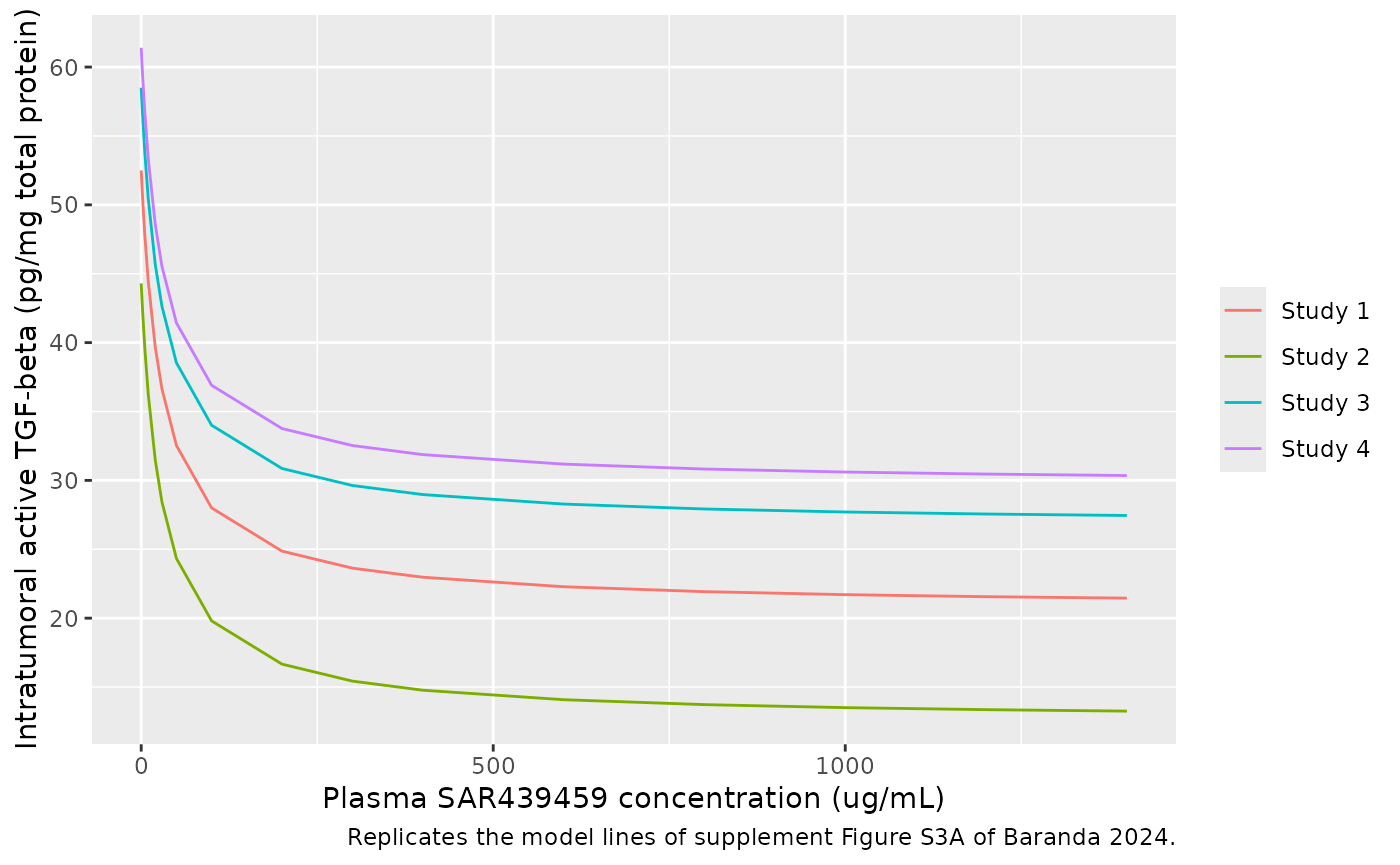
The typical lines in Figure S3A level off at about 21 (study 1), 13 (study 2), 27 (study 3) and 30 (study 4) pg/mg protein at 1400 ug/mL (digitised by the maintainers). The simulated values at 1400 ug/mL and at the EC50:
plateau <- sim_m |>
  filter(CP_SAR439459_MGL == 1400) |>
  select(study, tgfb_tumor) |>
  mutate(figure_s3a = c(21, 13, 27, 30))
plateau |>
  mutate(tgfb_tumor = signif(tgfb_tumor, 3)) |>
  dplyr::rename(
    Study = study,
    "Simulated at 1400 ug/mL" = tgfb_tumor,
    "Figure S3A (digitised)" = figure_s3a
  ) |>
knitr::kable()| Study | Simulated at 1400 ug/mL | Figure S3A (digitised) |
|---|---|---|
| Study 1 | 21.5 | 21 |
| Study 2 | 13.3 | 13 |
| Study 3 | 27.5 | 27 |
| Study 4 | 30.4 | 30 |
stopifnot(all(abs(plateau$tgfb_tumor - plateau$figure_s3a) < 3))

# At C = EC50 the decrease is Emax / 2 for every study; at 200 ug/mL the
# paper calls it 'close to 90% of Emax'. Same parameters on both sides, so
# these checks are exact up to floating point.
drop <- sim_m |>
  group_by(study) |>
  summarise(
    e0 = tgfb_tumor[CP_SAR439459_MGL == 0],
    at_ec50 = e0 - tgfb_tumor[CP_SAR439459_MGL == 29.4],
    at_200 = e0 - tgfb_tumor[CP_SAR439459_MGL == 200],
    .groups = "drop"
  )
stopifnot(
  all(abs(drop$at_ec50 - 31.7 / 2) < 1e-6),
  all(abs(drop$at_200 / 31.7 - 200 / (29.4 + 200)) < 1e-6),
  all(drop$at_200 / 31.7 > 0.85 & drop$at_200 / 31.7 < 0.90)
)
Human exposure against the mouse thresholds
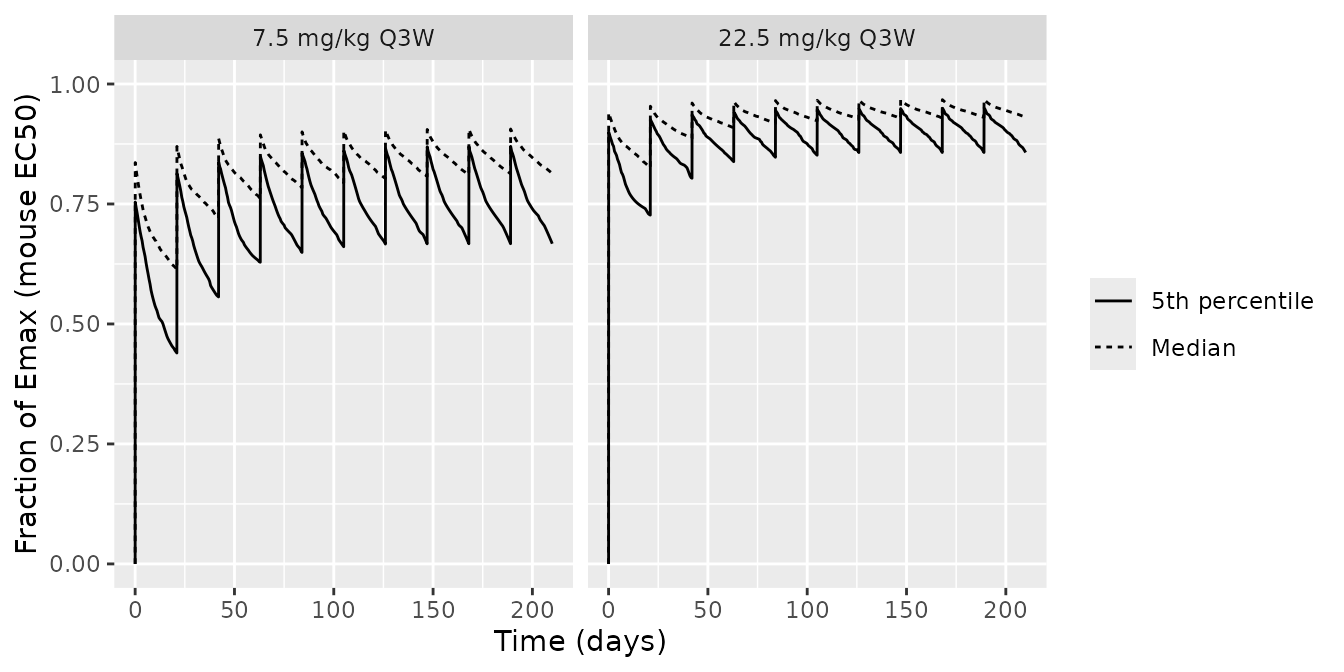
Supplement Figure S5 overlays the human simulations on the
mouse-derived thresholds. The fraction of the maximal intratumoral
TGF-beta decrease implied by the mouse EC50,
C / (EC50 + C), can be computed from the human median
profile. This is the source authors’ translational assumption (a mouse
plasma EC50 applied to human plasma), not a fitted human
relationship.
frac <- pct_h |>
  mutate(
    median_inhibition = p50 / (29.4 + p50),
    p05_inhibition = p05 / (29.4 + p05)
  )
ggplot(frac, aes(time)) +
  geom_line(aes(y = median_inhibition, linetype = "Median")) +
  geom_line(aes(y = p05_inhibition, linetype = "5th percentile")) +
  facet_wrap(~regimen) +
  scale_y_continuous(limits = c(0, 1)) +
  labs(
    x = "Time (days)", y = "Fraction of Emax (mouse EC50)", linetype = NULL
  )
Assumptions and deviations
- Reference weight. Table S2 gives the weight exponent on CL but not the value weight is centred on; 70 kg is assumed. The paper says covariate effects are expressed relative to the median, which is not reported.
- Weight distribution. Not reported; the virtual cohort uses a log-normal weight with median 70 kg and 20% CV, truncated to 40-130 kg.
- Infusion duration. Not reported; a 1-hour infusion is simulated. For a monoclonal antibody with a multi-day half-life this has no visible effect beyond the first hour.
- IIV. Table S2 reports Monolix omega (%) values; Monolix omega is the standard deviation of the log-normal random effect, so the variances are the squares (0.337^2, 0.224^2, 0.731^2). No correlations are reported.
-
Mouse Eq. 1. The equation in the supplement PDF is
garbled: it prints
TGFbeta = 0 - ...with the Emax fraction repeated three times. The intended formTGFbeta = E0 - Emax * C / (EC50 + C)follows from the text (‘direct Emax inhibition model’), from Table S3 reporting a separate E0 per study and a single Emax and EC50, and from the Figure S3A typical lines, which start at the per-study E0 and level off at E0 - Emax (checked above). -
Mouse PK. No mouse PK model is reported; the plasma
concentration is a per-record covariate column,
CP_SAR439459_MGL. The source fitted the measured plasma concentration paired with each tumour sample. - Mouse IIV. Table S3 reports no random effects; the model is typical-value plus proportional residual error.
- Figure S5 axis labels. In the 7.5 mg/kg panel the x-axis tick labels read 0, 21, 22, 23, 24, 105, … where the 22.5 mg/kg panel reads 0, 21, 42, 63, 84, 105, …; the two panels show the same Q3W schedule, so the 7.5 mg/kg labels are taken as a typographical error for 42, 63 and 84.
- Digitised values. Figure S5 medians and Figure S3A plateaus were read from the published figures and carry a few percent of reading error; the checks above allow for it.
-
Cemiplimab. Tested as a covariate and not retained
(‘Cemiplimab had no effect on SAR’459 PK exposure’); recorded under
covariatesDataExcluded.