Meropenem (Abulfathi 2021)
Source:vignettes/articles/Abulfathi_2021_meropenem.Rmd
Abulfathi_2021_meropenem.RmdModel and source
#> ℹ parameter labels from comments will be replaced by 'label()'Citation: Abulfathi AA, de Jager V, van Brakel E, Reuter H, Gupte N, Vanker N, Barnes GL, Nuermberger E, Dorman SE, Diacon AH, Dooley KE, Svensson EM. The Population Pharmacokinetics of Meropenem in Adult Patients With Rifampicin-Sensitive Pulmonary Tuberculosis. Front Pharmacol. 2021;12:637618. doi:10.3389/fphar.2021.637618
Description: Two-compartment population PK model for intravenous meropenem in South African adults with rifampicin-sensitive pulmonary tuberculosis (COMRADE trial; Abulfathi 2021). Allometric scaling on all disposition parameters with total body weight (reference 70 kg; fixed exponents 0.75 on CL and Q, 1 on V1 and V2) and a power effect of weight-standardised Cockcroft-Gault creatinine clearance (CRCL * 70 / WT, reference 115 mL/min) on CL; combined additive + proportional residual error.
Abulfathi and colleagues characterised the population pharmacokinetics of intravenous meropenem, which is being investigated for repurposing against tuberculosis, in adults with rifampicin-sensitive pulmonary tuberculosis enrolled in the phase 2 COMRADE trial. A two-compartment model with allometric weight scaling on all disposition parameters and a power effect of weight-standardised creatinine clearance on clearance described the data. Concomitant rifampicin and age had no significant effect on clearance.
Population
Sixty South African adults were randomised; the 49 who completed intensive pharmacokinetic sampling on day 14 form the analysis population (Abulfathi 2021 Table 1). Median age was 36.0 years (range 20.0-62.7), 24.5% were female, 32.7% were Black and 67.3% of mixed Asian ancestry, and 22.4% were HIV-positive. Median body weight was 52.7 kg (range 39.3-76.3; no patient was obese) and median Cockcroft-Gault creatinine clearance was 115 mL/min (range 57.7-203). Participants received meropenem for 14 days in one of four arms: 2 g over 0.5 h every 8 h with oral rifampicin 20 mg/kg once daily (MACR2X3, n = 12), 2 g over 0.5 h every 8 h (MAC2X3, n = 13), 1 g over 0.5 h every 8 h (MAC1X3, n = 12), or 3 g over 1 h once daily (MAC3X1, n = 12). All arms also received oral amoxicillin/clavulanate with each meropenem dose. Samples were taken pre-dose and at 0.5, 1, 1.5, 2, 3, 4, 6 and 8 h after the day-14 dose; 404 of 441 concentrations were analysed (LLOQ 0.5 mg/L).
The same information is available programmatically via
readModelDb("Abulfathi_2021_meropenem")()$population.
Source trace
The per-parameter origin is recorded as an in-file comment next to
each ini() entry in
inst/modeldb/specificDrugs/Abulfathi_2021_meropenem.R. The
covariate equations are printed in NONMEM syntax in the footnote of
Abulfathi 2021 Table 2.
| Equation / parameter | Value | Source location |
|---|---|---|
lcl (CL, L/h per 70 kg) |
log(11.8) | Table 2 |
lvc (V1, L per 70 kg) |
log(14.2) | Table 2 |
lq (Q, L/h per 70 kg) |
log(3.26) | Table 2 |
lvp (V2, L per 70 kg) |
log(3.12) | Table 2 |
e_wt_cl_q |
0.75 (fixed) | Results; Table 2 footnote (TVCL, TVQ) |
e_wt_vc_vp |
1 (fixed) | Results; Table 2 footnote (TVV1,
TVV2) |
e_crcl_cl |
0.416 | Table 2 (‘Creatinine clearance on CL’); footnote
THETA(7)
|
etalcl |
log(0.20^2 + 1) = 0.0392 | Table 2 (20 %CV); footnote b
(%CV = SQRT(EXP(OMEGA)-1)*100) |
etalvc |
log(0.131^2 + 1) = 0.0170 | Table 2 (13.1 %CV) |
etalvp |
log(1.06^2 + 1) = 0.7531 | Table 2 (106 %CV) |
propSd |
0.178 | Table 2 (‘Proportional residual error’) |
addSd |
1.16 mg/L | Table 2 (‘Additive residual error’) |
cl = CL * (WT/70)^0.75 * ((CRCL*70/WT)/115)^0.416 |
n/a | Table 2 footnote TVCL
|
vc = V1 * WT/70, q = Q * (WT/70)^0.75,
vp = V2 * WT/70
|
n/a | Table 2 footnote TVV1, TVQ,
TVV2
|
| Two-compartment ODEs with elimination from central | n/a | Figure 2 (structural schema) |
Deterministic checks of the covariate model
The reference subject (70 kg, creatinine clearance 115 mL/min, so the weight-standardised value is also 115 mL/min) must have the published typical clearance of 11.8 L/h. The Discussion also states that “in a 70 kg patient with severe renal impairment (CLCR of 5-30 ml/min), about a 40-70% reduction in meropenem doses would be required”, which follows from the ratio of clearances.
mod <- readModelDb("Abulfathi_2021_meropenem")
mod_typical <- rxode2::zeroRe(mod)
#> ℹ parameter labels from comments will be replaced by 'label()'

cl_at <- function(wt, crcl) {
  ev <- data.frame(id = 1, time = 0, evid = 0, cmt = "central", WT = wt, CRCL = crcl)
  rxode2::rxSolve(mod_typical, ev, returnType = "data.frame")$cl
}

cl_ref <- cl_at(70, 115)
#> ℹ omega/sigma items treated as zero: 'etalcl', 'etalvc', 'etalvp'
renal <- tibble::tibble(
  CRCL = c(5, 30, 115),
  cl = vapply(CRCL, function(x) cl_at(70, x), numeric(1)),
  reduction_pct = 100 * (1 - cl / cl_ref)
)
#> ℹ omega/sigma items treated as zero: 'etalcl', 'etalvc', 'etalvp'
#> ℹ omega/sigma items treated as zero: 'etalcl', 'etalvc', 'etalvp'
#> ℹ omega/sigma items treated as zero: 'etalcl', 'etalvc', 'etalvp'
knitr::kable(renal, digits = 2, caption = "Typical CL for a 70 kg patient by creatinine clearance.")| CRCL | cl | reduction_pct |
|---|---|---|
| 5 | 3.20 | 72.87 |
| 30 | 6.75 | 42.82 |
| 115 | 11.80 | 0.00 |
stopifnot(
  abs(cl_ref / 11.8 - 1) < 1e-8,
  # Paper: 'about a 40-70% reduction' across CLCR 5-30 mL/min.
  renal$reduction_pct[renal$CRCL == 30] > 35, renal$reduction_pct[renal$CRCL == 30] < 50,
  renal$reduction_pct[renal$CRCL == 5] > 65, renal$reduction_pct[renal$CRCL == 5] < 80
)
The model gives a 43% reduction at 30 mL/min and a 73% reduction at 5 mL/min, in line with the paper’s “about 40-70%”.
Typical-value profiles against the observed medians of Figure 4
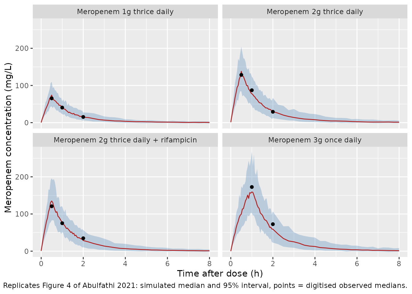
Figure 4 of the paper overlays the observed median concentration (solid red line) for each arm on day 14. The maintainers digitised that line from the figure image at 0.5, 1 and 2 h after the dose. The table below compares it with the typical-value prediction for a subject at the population median weight (52.7 kg) and creatinine clearance (115 mL/min) after 14 days of dosing. The two are not the same quantity (a median of 12-13 observed patients versus one typical subject), so the check is a structural one: a mis-transcribed clearance, volume, dose or unit moves every point by tens of percent.
arms <- tibble::tribble(
  ~arm,                          ~amt, ~dur, ~tau,
  "Meropenem 1g thrice daily",   1000, 0.5,  8,
  "Meropenem 2g thrice daily",   2000, 0.5,  8,
  "Meropenem 2g thrice daily + rifampicin", 2000, 0.5, 8,
  "Meropenem 3g once daily",     3000, 1.0,  24
)
day14 <- 13 * 24 # start of the day-14 dosing interval (h)

make_events <- function(ids, wt, crcl, arm_row, obs_times) {
  n_dose <- 14 * 24 / arm_row$tau
  subj <- tibble::tibble(id = ids, WT = wt, CRCL = crcl, arm = arm_row$arm)
  doses <- subj |>
    tidyr::crossing(time = (seq_len(n_dose) - 1) * arm_row$tau) |>
    dplyr::mutate(
      evid = 1L, cmt = "central", amt = arm_row$amt,
      rate = arm_row$amt / arm_row$dur, dose_time = time
    ) |>
    dplyr::filter(time <= day14)
  obs <- subj |>
    tidyr::crossing(tad = obs_times) |>
    dplyr::mutate(
      time = day14 + tad, evid = 0L, cmt = "central",
      amt = NA_real_, rate = NA_real_
    ) |>
    dplyr::select(-tad)
  dplyr::bind_rows(doses, obs) |>
    dplyr::select(id, time, evid, cmt, amt, rate, WT, CRCL, arm) |>
    dplyr::arrange(id, time, dplyr::desc(evid))
}

ev_typ <- dplyr::bind_rows(lapply(seq_len(nrow(arms)), function(i) {
  make_events(i, 52.7, 115, arms[i, ], obs_times = seq(0, 8, by = 0.05))
}))
sim_typ <- rxode2::rxSolve(mod_typical, ev_typ, keep = "arm", returnType = "data.frame") |>
  dplyr::mutate(tad = time - day14)
#> ℹ omega/sigma items treated as zero: 'etalcl', 'etalvc', 'etalvp'
#> Warning: multi-subject simulation without without 'omega'

# Observed medians digitised from Figure 4 (solid red line), mg/L.
fig4_obs <- tibble::tribble(
  ~arm,                                     ~tad, ~obs_median,
  "Meropenem 1g thrice daily",               0.5,  65.3,
  "Meropenem 1g thrice daily",               1.0,  40.5,
  "Meropenem 1g thrice daily",               2.0,  15.3,
  "Meropenem 2g thrice daily",               0.5, 128.5,
  "Meropenem 2g thrice daily",               1.0,  87.2,
  "Meropenem 2g thrice daily",               2.0,  29.2,
  "Meropenem 2g thrice daily + rifampicin",  0.5, 120.8,
  "Meropenem 2g thrice daily + rifampicin",  1.0,  75.2,
  "Meropenem 2g thrice daily + rifampicin",  2.0,  34.7,
  "Meropenem 3g once daily",                 1.0, 172.6,
  "Meropenem 3g once daily",                 2.0,  72.6
)

cmp_typ <- fig4_obs |>
  dplyr::left_join(
    sim_typ |> dplyr::mutate(tad = round(tad, 2)) |> dplyr::select(arm, tad, Cc),
    by = c("arm", "tad")
  ) |>
  dplyr::mutate(pct_diff = 100 * (Cc / obs_median - 1))
stopifnot(nrow(cmp_typ) == nrow(fig4_obs), !anyNA(cmp_typ$Cc))

cmp_typ |>
  dplyr::rename(
    "Arm" = arm, "Time after dose (h)" = tad,
    "Observed median, Fig. 4 (mg/L)" = obs_median,
    "Typical-value Cc (mg/L)" = Cc, "Difference (%)" = pct_diff
  ) |>
knitr::kable(digits = 1, caption = "Typical-value prediction versus digitised observed medians (Figure 4).")| Arm | Time after dose (h) | Observed median, Fig. 4 (mg/L) | Typical-value Cc (mg/L) | Difference (%) |
|---|---|---|---|---|
| Meropenem 1g thrice daily | 0.5 | 65.3 | 70.4 | 7.8 |
| Meropenem 1g thrice daily | 1.0 | 40.5 | 40.3 | -0.5 |
| Meropenem 1g thrice daily | 2.0 | 15.3 | 15.8 | 3.5 |
| Meropenem 2g thrice daily | 0.5 | 128.5 | 140.9 | 9.6 |
| Meropenem 2g thrice daily | 1.0 | 87.2 | 80.6 | -7.6 |
| Meropenem 2g thrice daily | 2.0 | 29.2 | 31.7 | 8.5 |
| Meropenem 2g thrice daily + rifampicin | 0.5 | 120.8 | 140.9 | 16.6 |
| Meropenem 2g thrice daily + rifampicin | 1.0 | 75.2 | 80.6 | 7.2 |
| Meropenem 2g thrice daily + rifampicin | 2.0 | 34.7 | 31.7 | -8.7 |
| Meropenem 3g once daily | 1.0 | 172.6 | 165.6 | -4.1 |
| Meropenem 3g once daily | 2.0 | 72.6 | 60.4 | -16.8 |
# Deterministic solve, so the bounds are not cohort-dependent. Measured median
# difference +3.5%, largest |difference| 16.8% (3 g arm at 2 h). The residual
# gap is the typical subject versus a 12-13 patient observed median.
stopifnot(
  abs(median(cmp_typ$pct_diff)) < 10,
  max(abs(cmp_typ$pct_diff)) < 25
)
Virtual cohort
Observed data are not publicly available. The virtual cohort draws body weight and creatinine clearance independently from log-normal distributions matched to the Table 1 medians and interquartile ranges. Values outside the observed ranges are redrawn rather than clipped. Each arm has 100 subjects.
set.seed(20210629)
rtrunc_lnorm <- function(n, median, q1, q3, lo, hi) {
  sdlog <- (log(q3) - log(q1)) / (2 * qnorm(0.75))
  out <- numeric(0)
  while (length(out) < n) {
    x <- rlnorm(n, log(median), sdlog)
    out <- c(out, x[x >= lo & x <= hi])
  }
  out[seq_len(n)]
}

n_per_arm <- 100
events <- dplyr::bind_rows(lapply(seq_len(nrow(arms)), function(i) {
  ids <- (i - 1) * n_per_arm + seq_len(n_per_arm)
  make_events(
    ids,
    wt = rtrunc_lnorm(n_per_arm, 52.7, 47.5, 57.1, 39.3, 76.3),
    crcl = rtrunc_lnorm(n_per_arm, 115, 94.3, 137, 57.7, 203),
    arms[i, ],
    obs_times = c(seq(0, 2, by = 0.05), seq(2.25, 8, by = 0.25),
                  if (arms$tau[i] == 24) seq(9, 24, by = 1))
  )
}))
stopifnot(!anyDuplicated(unique(events[, c("id", "time", "evid")])))Replicate Figure 4 (visual predictive check)
The simulated 2.5th, 50th and 97.5th percentiles include residual
error (the sim column). The points are the observed medians
digitised from Figure 4.
sim |>
  dplyr::filter(tad <= 8) |>
  dplyr::group_by(arm, tad) |>
  dplyr::summarise(
    lo = quantile(sim, 0.025), med = median(sim), hi = quantile(sim, 0.975),
    .groups = "drop"
  ) |>
  ggplot(aes(tad, med)) +
  geom_ribbon(aes(ymin = lo, ymax = hi), fill = "steelblue", alpha = 0.3) +
  geom_line(colour = "firebrick") +
  geom_point(data = fig4_obs, aes(tad, obs_median), inherit.aes = FALSE) +
  facet_wrap(~arm) +
  labs(
    x = "Time after dose (h)", y = "Meropenem concentration (mg/L)",
    caption = paste(
      "Replicates Figure 4 of Abulfathi 2021: simulated median and 95% interval,",
      "points = digitised observed medians."
    )
  )
PKNCA validation
Non-compartmental analysis of the day-14 dosing interval (individual predictions, no residual error). The paper reports no NCA table, so the check here is internal: at steady state the dosing-interval AUC must equal dose / CL for each simulated subject.
sim_nca <- sim |>
  dplyr::filter(!is.na(Cc)) |>
  dplyr::mutate(time = tad) |>
  dplyr::select(id, time, Cc, arm)
# The day-14 observation grid starts at the dose time (time after dose 0), so
# every subject already carries the time-zero record PKNCA needs.
stopifnot(all(tapply(sim_nca$time, sim_nca$id, min) == 0))

dose_df <- events |>
  dplyr::filter(evid == 1, time == day14) |>
  dplyr::mutate(time = 0) |>
  dplyr::select(id, time, amt, arm)

conc_obj <- PKNCA::PKNCAconc(sim_nca, Cc ~ time | arm + id)
dose_obj <- PKNCA::PKNCAdose(dose_df, amt ~ time | arm + id)
intervals <- dplyr::bind_rows(
  data.frame(start = 0, end = 8, arm = arms$arm[arms$tau == 8],
             cmax = TRUE, tmax = TRUE, auclast = TRUE, cmin = TRUE),
  data.frame(start = 0, end = 24, arm = arms$arm[arms$tau == 24],
             cmax = TRUE, tmax = TRUE, auclast = TRUE, cmin = TRUE)
)
nca_res <- PKNCA::pk.nca(PKNCA::PKNCAdata(conc_obj, dose_obj, intervals = intervals))

nca_wide <- as.data.frame(nca_res$result) |>
  dplyr::select(id, arm, PPTESTCD, PPORRES) |>
  tidyr::pivot_wider(names_from = PPTESTCD, values_from = PPORRES)

nca_wide |>
  dplyr::group_by(arm) |>
  dplyr::summarise(
    cmax = median(cmax), tmax = median(tmax),
    auclast = median(auclast), cmin = median(cmin), .groups = "drop"
  ) |>
  dplyr::rename(
    "Arm" = arm, "Cmax (mg/L)" = cmax, "Tmax (h)" = tmax,
    "AUCtau (mg*h/L)" = auclast, "Cmin (mg/L)" = cmin
  ) |>
knitr::kable(digits = 2, caption = "Median simulated day-14 NCA by arm.")| Arm | Cmax (mg/L) | Tmax (h) | AUCtau (mg*h/L) | Cmin (mg/L) |
|---|---|---|---|---|
| Meropenem 1g thrice daily | 71.72 | 0.5 | 94.86 | 0.33 |
| Meropenem 2g thrice daily | 137.25 | 0.5 | 188.51 | 0.87 |
| Meropenem 2g thrice daily + rifampicin | 137.55 | 0.5 | 187.90 | 0.73 |
| Meropenem 3g once daily | 164.26 | 1.0 | 289.32 | 0.00 |
cl_ind <- sim |>
  dplyr::filter(tad == 0) |>
  dplyr::distinct(id, cl)
auc_chk <- nca_wide |>
  dplyr::left_join(cl_ind, by = "id") |>
  dplyr::left_join(dose_df |> dplyr::select(id, amt), by = "id") |>
  dplyr::mutate(pct_diff = 100 * (auclast * cl / amt - 1))
stopifnot(nrow(auc_chk) == 4 * n_per_arm, !anyNA(auc_chk$pct_diff))
summary(auc_chk$pct_diff)
#>      Min.   1st Qu.    Median      Mean   3rd Qu.      Max.
#> -0.048316 -0.011322 -0.004460 -0.004957  0.002549  0.017004

# Trapezoidal error on a 0.05 h grid around the infusion peak; the two sides
# use the same drawn parameters, so the gap is numerical (measured: median
# -0.004%, all subjects within 0.05%). A wrong dose, unit or clearance breaks
# this by far more than the bounds.
stopifnot(
  abs(median(auc_chk$pct_diff)) < 0.5,
  max(abs(auc_chk$pct_diff)) < 1
)
Assumptions and deviations
- Residual error scale. Table 2 lists the proportional error as “0.178” under a “(%)” header and the additive error as “1.16” in mg/L. Both are taken as standard deviations (17.8% and 1.16 mg/L), since a variance would carry squared units. The paper does not print the error equation. The combined error is encoded in nlmixr2’s default additive-plus-proportional form (variances summed).
-
Creatinine clearance.
CRCLis the raw Cockcroft-Gault creatinine clearance in mL/min, not the BSA-normalised mL/min/1.73 m^2 form of the canonical column. The model divides it by weight/70 internally, exactly as in the Table 2 footnote (CLCR*70/WTKG). Users must supply the raw value. - Virtual cohort. Weight and creatinine clearance are drawn independently, although Cockcroft-Gault clearance correlates with weight. Age, sex and serum creatinine are not needed by the final model.
- Rifampicin arm. The final model has no rifampicin effect, so the MACR2X3 and MAC2X3 arms share the same simulated exposure distribution.
- Figure 4 targets. The observed medians were digitised by the maintainers from the published Figure 4 image (pixel coordinates calibrated to the axis ticks). Precision is about +/- 2 mg/L.
- Supplement. The supplementary data sheet (eligibility criteria, bioanalytical method, individual fits and residual diagnostics) could not be retrieved. The article states it contains no model parameters; all values come from the main text and Table 2.
- No erratum or correction notice was found for this article (checked 2026-09-28).