Ixekizumab (Jackson 2022)
Source:vignettes/articles/Jackson_2022_ixekizumab.Rmd
Jackson_2022_ixekizumab.Rmd
library(nlmixr2lib)
library(rxode2)
#> rxode2 5.1.2 using 2 threads (see ?getRxThreads)
#>   no cache: create with `rxCreateCache()`
library(dplyr)
#>
#> Attaching package: 'dplyr'
#> The following objects are masked from 'package:stats':
#>
#>     filter, lag
#> The following objects are masked from 'package:base':
#>
#>     intersect, setdiff, setequal, union
library(tidyr)
library(ggplot2)
library(PKNCA)
#>
#> Attaching package: 'PKNCA'
#> The following object is masked from 'package:stats':
#>
#>     filter
Ixekizumab paediatric population PK (IXORA-PEDS)
Simulate ixekizumab serum concentration–time profiles using the final paediatric population PK model of Jackson et al. (2022) for patients aged 6 to <18 years with moderate-to-severe plaque psoriasis enrolled in IXORA-PEDS (NCT03073200). The model is a two-compartment linear PK model with first-order subcutaneous absorption, an allometric body-weight effect on CL, Q, V2, and V3, and a log-linear ADA-titre effect on CL.
- Citation: Jackson K, Chua L, Velez de Mendizabal N, et al. Population pharmacokinetic and exposure-efficacy analysis of ixekizumab in paediatric patients with moderate-to-severe plaque psoriasis (IXORA-PEDS). Br J Clin Pharmacol. 2022;88(3):1074-1086. doi:10.1111/bcp.15034
- Article: https://doi.org/10.1111/bcp.15034
Population
IXORA-PEDS is a Phase 3, double-blind, placebo-controlled trial conducted in paediatric patients aged 6 to <18 years with moderate-to-severe plaque psoriasis (PASI ≥ 12, sPGA ≥ 3, BSA ≥ 10% at screening and baseline). The population PK analysis dataset comprised 558 measurable ixekizumab serum concentrations from 184 patients: 4 patients <25 kg (2.2%), 45 patients 25–50 kg (24.5%), and 135 patients >50 kg (73.4%). Overall baseline age ranged 6–17 years (median 15 years in the >50 kg group, 10 years in the 25–50 kg group, 7 years in the <25 kg group), baseline weight 21.5–136 kg, 56.5% female. The majority were white (81.5%), with 3.26% Black/African American, 3.26% Asian, 1.63% American Indian or Alaska Native, 7.61% Other, and 2.72% missing race. Regions: US 37.5%, Europe 41.3%, Rest of World 21.2%. Baseline demographics reproduced from Jackson 2022 Table 1. The approved weight-based Q4W regimens are 20 mg (<25 kg), 40 mg (25–50 kg), and 80 mg (>50 kg), after an initial 40/80/160 mg loading dose respectively.
Programmatic access:
readModelDb("Jackson_2022_ixekizumab")$population.
Source trace
| Equation / parameter | Value | Source location |
|---|---|---|
| Two-compartment linear model with first-order SC absorption | structural | Jackson 2022 Methods section 2.5 and Table 2 header |
| Ka | 0.00801 h-1 | Table 2 (Rate of absorption) |
| CL (reference 58.6 kg, ADA-negative) | 0.0120 L/h | Table 2 (Clearance) |
| Q (reference 58.6 kg) | 0.0119 L/h | Table 2 (Clearance) |
| V2 (reference 58.6 kg) | 2.72 L | Table 2 (Volume of distribution) |
| V3 (reference 58.6 kg) | 2.11 L | Table 2 (Volume of distribution) |
| F1 | 0.72 (FIXED) | Table 2 + footnote c (fixed to adult model value) |
| Allometric exponent on CL and Q | 0.989 | Table 2 (Covariate weight on CL and Q) |
| Allometric exponent on V2 and V3 | 0.998 | Table 2 (Covariate weight on V2 and V3) |
| ADA-titre coefficient on CL | 0.0292 | Table 2 (Covariate ADA titre on CL) |
| CL covariate equation | CL*(WT/58.6)^0.989*(1 + 0.0292*log_e[ADA titre]) |
Table 2 footnote (CL_individual equation) |
| Q covariate equation | Q*(WT/58.6)^0.989 |
Table 2 footnote (Q_individual equation) |
| V2 covariate equation | V2*(WT/58.6)^0.998 |
Table 2 footnote (V2,individual equation) |
| V3 covariate equation | V3*(WT/58.6)^0.998 |
Table 2 footnote (V3,individual equation) |
| IIV on CL | 28.4% (ω² = log(1 + 0.284²) = 0.0776) | Table 2 (Interindividual variability column) + footnote b (%IIV = 100·√(e^OMEGA − 1)) |
| Residual error (proportional) | 27.7% | Table 2 (Residual error (proportional)) |
| Approved Q4W weight-based dosing (20/40/80 mg with loading 40/80/160 mg) | regimen | Introduction, page 1075, and Methods section 2.1 |
| Reported steady-state (Week 8 and Week 12) mean trough concentrations | 3.20–3.33 µg/mL (25–50 and >50 kg groups) | Results section 3.1, first paragraph |
| Reported normalized 70-kg CL / Vss | 0.0144 L/h / 5.77 L | Discussion, page 1083 |
| Reported mean terminal half-life | ~12 days | Discussion, page 1083 |
Covariate column naming
| Source column | Canonical column used here |
|---|---|
WT (baseline body weight, kg) |
WT |
ADA titre (continuous reciprocal dilution; 1:10, 1:20,
…, 1:2560) |
ADA_TITER (per
inst/references/covariate-columns.md). ADA-negative samples
encoded as ADA_TITER = 1 so that log_e(1) = 0
cancels the covariate effect (85.8% of the dataset). |
Virtual cohort
The IXORA-PEDS patient-level data are not publicly available, so the figures below use a virtual paediatric cohort whose weight, weight-group, and ADA distributions approximate Jackson 2022 Table 1 and the ADA incidence reported in Results section 3.1.
set.seed(20220301) # IXORA-PEDS paper month
n_subj <- 184 # match dataset size

# Weight-group proportions from Jackson 2022 Table 1 (overall column)
# <25 kg: 4/184 = 2.2%; 25-50 kg: 45/184 = 24.5%; >50 kg: 135/184 = 73.4%
u <- runif(n_subj)
weight_group <- cut(
  u,
  breaks = c(-Inf, 4 / 184, 49 / 184, Inf),
  labels = c("<25 kg", "25-50 kg", ">50 kg"),
  right  = TRUE
)

# Sample body weights inside each group to match the reported mean +/- SD
# from Jackson 2022 Table 1. Clip to the reported per-group ranges.
simulate_weight <- function(group) {
  switch(as.character(group),
    "<25 kg"   = pmin(22.6, pmax(21.5, rnorm(1, 21.9, 0.520))),
    "25-50 kg" = pmin(50.0, pmax(25.0, rnorm(1, 37.7, 8.10))),
    ">50 kg"   = pmin(136.0, pmax(50.1, rnorm(1, 71.3, 19.5)))
  )
}
WT <- vapply(weight_group, simulate_weight, numeric(1))

# ADA titre: 85.8% ADA-negative (ADA_TITER = 1); 14.2% TE-ADA-positive with
# titres in three bands per Results section 3.1:
#   - Low    (<1:160)        : 52.6% of ADA+ samples
#   - Moderate (>=1:160, <1:1280): 38.5%
#   - High     (>=1:1280)    :  9.0%
ada_pos <- runif(n_subj) < 0.142
ada_titre <- rep(1, n_subj)
n_pos <- sum(ada_pos)
if (n_pos > 0) {
  band <- sample(c("low", "mod", "high"),
    size    = n_pos,
    replace = TRUE,
    prob    = c(0.526, 0.385, 0.090)
  )
  titre_sample <- function(b) {
    switch(b,
      low  = sample(c(10, 20, 40, 80), 1),          # 1:10 to <1:160
      mod  = sample(c(160, 320, 640), 1),           # 1:160 to <1:1280
      high = sample(c(1280, 2560), 1)               # >=1:1280
    )
  }
  ada_titre[ada_pos] <- vapply(band, titre_sample, numeric(1))
}

cohort <- tibble(
  ID           = seq_len(n_subj),
  weight_group = weight_group,
  WT           = WT,
  ADA_TITER    = ada_titre
)

summary_tbl <- cohort |>
  group_by(weight_group) |>
  summarise(
    n           = dplyr::n(),
    mean_WT     = mean(WT),
    median_WT   = median(WT),
    pct_ada_pos = 100 * mean(ADA_TITER > 1),
    .groups     = "drop"
  )
knitr::kable(summary_tbl, digits = 2,
caption = "Simulated cohort summary (compare with Jackson 2022 Table 1 weight-group means and Results 3.1 ADA incidence).")| weight_group | n | mean_WT | median_WT | pct_ada_pos |
|---|---|---|---|---|
| <25 kg | 9 | 21.91 | 21.86 | 22.22 |
| 25-50 kg | 43 | 38.99 | 40.04 | 11.63 |
| >50 kg | 132 | 74.64 | 73.96 | 12.12 |
Dosing dataset
Weight-based Q4W regimen per IXORA-PEDS: loading dose at Week 0 (40/80/160 mg for <25/25–50/>50 kg), then maintenance Q4W (20/40/80 mg). Simulate through Week 24 (6 maintenance doses) so that the trough at Week 12 (the co-primary endpoint timepoint) reflects steady state. Times are in hours (model unit).
# Weeks -> hours conversion
hours_per_week <- 7 * 24

maint_doses <- function(group) {
  switch(as.character(group), "<25 kg" = 20, "25-50 kg" = 40, ">50 kg" = 80)
}
load_doses <- function(group) {
  switch(as.character(group), "<25 kg" = 40, "25-50 kg" = 80, ">50 kg" = 160)
}

dose_weeks    <- c(0, 4, 8, 12, 16, 20)
dose_times_hr <- dose_weeks * hours_per_week
obs_weeks     <- sort(unique(c(seq(0, 24, by = 0.5), 1, 9))) # dense early + the Week 1 and Week 9 PK addendum timepoints
obs_times_hr  <- obs_weeks * hours_per_week

d_dose <- cohort |>
  tidyr::crossing(dose_idx = seq_along(dose_times_hr)) |>
  mutate(
    TIME = dose_times_hr[dose_idx],
    AMT  = ifelse(dose_idx == 1,
                  vapply(weight_group, load_doses, numeric(1)),
                  vapply(weight_group, maint_doses, numeric(1))),
    EVID = 1,
    CMT  = "depot",
    DV   = NA_real_
  ) |>
  select(-dose_idx)

d_obs <- cohort |>
  tidyr::crossing(TIME = obs_times_hr) |>
  mutate(
    AMT  = 0,
    EVID = 0,
    CMT  = "central",
    DV   = NA_real_
  )

d_sim <- bind_rows(d_dose, d_obs) |>
  arrange(ID, TIME, desc(EVID)) |>
  as.data.frame()
Simulation
mod <- readModelDb("Jackson_2022_ixekizumab")
set.seed(42)
# `weight_group` and `WT` are per-subject columns already on every row of
# `d_sim` (built from `cohort |> tidyr::crossing(...)`). Carrying them
# through `rxSolve(keep = ...)` removes the need for post-rxSolve
# left_joins from `cohort` in every downstream chunk.
sim <- rxode2::rxSolve(mod, events = d_sim, returnType = "data.frame",
                       keep = c("weight_group", "WT"))
#> ℹ parameter labels from comments will be replaced by 'label()'
Replicate published figures
Figure 1 — Mean ixekizumab concentration vs time by weight group (Weeks 0–12)
Jackson 2022 Figure 1 plots mean (±SD) trough-only observed concentrations in the 25–50 kg and >50 kg groups through Week 12. The simulated curves below show the mean (and 5th/95th percentile ribbon) of simulated ixekizumab concentrations over the same window, stratified by baseline weight group.
sim_plot <- sim |>
  as.data.frame() |>
  filter(time > 0, time <= 12 * hours_per_week, !is.na(Cc)) |>
  mutate(week = time / hours_per_week)

fig1 <- sim_plot |>
  group_by(weight_group, week) |>
  summarise(
    mean_Cc = mean(Cc, na.rm = TRUE),
    Q05     = quantile(Cc, 0.05, na.rm = TRUE),
    Q95     = quantile(Cc, 0.95, na.rm = TRUE),
    .groups = "drop"
  )

ggplot(fig1, aes(x = week, y = mean_Cc, colour = weight_group, fill = weight_group)) +
  geom_ribbon(aes(ymin = Q05, ymax = Q95), alpha = 0.15, colour = NA) +
  geom_line(linewidth = 0.9) +
  scale_y_continuous() +
  scale_x_continuous(breaks = seq(0, 12, by = 4)) +
  labs(
    x = "Time (weeks)",
    y = "Ixekizumab concentration (\u03bcg/mL)",
    title = "Figure 1 replication: mean concentration by weight group",
    subtitle = "Simulated Weeks 0\u201312 (loading + Q4W maintenance); mean and 5\u201395th percentile",
    caption = "Replicates Figure 1 of Jackson 2022."
  ) +
  theme_bw()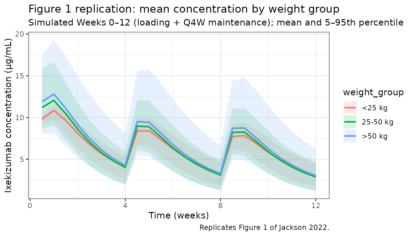
Figure 3A — Week 12 trough concentration vs body weight
wk12_time <- 12 * hours_per_week
sim_wk12 <- sim |>
  as.data.frame() |>
  filter(abs(time - wk12_time) < 1e-6)

ggplot(sim_wk12, aes(x = WT, y = Cc, colour = weight_group)) +
  geom_point(alpha = 0.5) +
  scale_y_log10() +
  labs(
    x = "Baseline body weight (kg)",
    y = "Week 12 trough concentration (\u03bcg/mL)",
    title = "Figure 3A replication: Week 12 model-predicted trough vs body weight",
    caption = "Replicates Figure 3A of Jackson 2022."
  ) +
  theme_bw()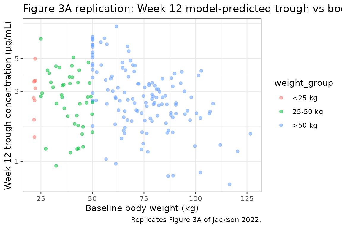
Steady-state trough by weight group (Weeks 8 and 12)
Jackson 2022 Results section 3.1 reports mean trough concentrations at predicted steady state (Weeks 8 and 12) in the 25–50 kg and >50 kg groups in the range 3.20–3.33 µg/mL. Insufficient PK data were available to summarise the <25 kg group.
trough_weeks <- c(8, 12)
trough_times <- trough_weeks * hours_per_week

trough_tbl <- sim |>
  as.data.frame() |>
  filter(time %in% trough_times) |>
  group_by(weight_group, week = time / hours_per_week) |>
  summarise(
    mean_trough  = mean(Cc, na.rm = TRUE),
    sd_trough    = sd(Cc, na.rm = TRUE),
    median_trough = median(Cc, na.rm = TRUE),
    .groups      = "drop"
  )

knitr::kable(trough_tbl, digits = 2,
             caption = paste(
               "Simulated mean trough concentrations at Weeks 8 and 12.",
               "Compare with Jackson 2022 Results 3.1: reported means 3.20\u20133.33 \u03bcg/mL",
               "in the 25\u201350 kg and >50 kg groups; insufficient data in the <25 kg group."
))| weight_group | week | mean_trough | sd_trough | median_trough |
|---|---|---|---|---|
| <25 kg | 8 | 2.54 | 1.23 | 2.17 |
| <25 kg | 12 | 2.36 | 1.20 | 1.99 |
| 25-50 kg | 8 | 3.28 | 1.48 | 2.80 |
| 25-50 kg | 12 | 3.05 | 1.44 | 2.57 |
| >50 kg | 8 | 3.52 | 1.53 | 3.49 |
| >50 kg | 12 | 3.27 | 1.46 | 3.23 |
PKNCA validation
Run PKNCA on the steady-state dosing interval between the Week 8 and Week 12 doses (i.e., from the Week 8 dose to the Week 12 dose, a 4-week window). This is the interval over which Jackson 2022 reports steady-state trough concentrations.
ss_start <- 8  * hours_per_week
ss_end   <- 12 * hours_per_week

nca_conc <- sim |>
  as.data.frame() |>
  filter(time >= ss_start, time <= ss_end) |>
  mutate(time_rel = time - ss_start,
         treatment = paste0("IXE_Q4W_", weight_group)) |>
  rename(ID = id) |>
  select(ID, time_rel, Cc, treatment)

nca_dose <- cohort |>
  mutate(time_rel = 0,
         AMT      = vapply(weight_group, maint_doses, numeric(1)),
         treatment = paste0("IXE_Q4W_", weight_group)) |>
  select(ID, time_rel, AMT, treatment)

conc_obj <- PKNCAconc(nca_conc, Cc ~ time_rel | treatment + ID)
dose_obj <- PKNCAdose(nca_dose, AMT ~ time_rel | treatment + ID)

data_obj <- PKNCAdata(
  conc_obj,
  dose_obj,
  intervals = data.frame(
    start   = 0,
    end     = 4 * hours_per_week,
    cmax    = TRUE,
    tmax    = TRUE,
    cmin    = TRUE,
    auclast = TRUE,
    cav     = TRUE
  )
)

nca_results <- pk.nca(data_obj)
nca_summary <- summary(nca_results)
knitr::kable(
  nca_summary,
  digits  = 2,
  caption = paste(
    "Simulated steady-state (Week 8\u2013Week 12) NCA by weight group.",
    "Cmin is the trough at Week 12; compare with Jackson 2022 Results 3.1:",
    "reported mean trough 3.20\u20133.33 \u03bcg/mL in the 25\u201350 and >50 kg groups."
  )
)| start | end | treatment | N | auclast | cmax | cmin | tmax | cav |
|---|---|---|---|---|---|---|---|---|
| 0 | 672 | IXE_Q4W_<25 kg | 9 | 3030 [27.3] | 6.85 [19.0] | 2.15 [45.1] | 84.0 [84.0, 168] | 4.50 [27.3] |
| 0 | 672 | IXE_Q4W_>50 kg | 132 | 3960 [35.5] | 8.77 [29.2] | 2.94 [51.6] | 168 [84.0, 168] | 5.89 [35.5] |
| 0 | 672 | IXE_Q4W_25-50 kg | 43 | 3730 [31.0] | 8.28 [24.9] | 2.77 [47.0] | 168 [84.0, 168] | 5.55 [31.0] |
Comparison against published troughs
pub <- tibble(
  weight_group = c("<25 kg", "25-50 kg", ">50 kg"),
  published_mean_trough = c(
    NA_real_,  # insufficient data in <25 kg group
    mean(c(3.20, 3.33)),
    mean(c(3.20, 3.33))
  ),
  published_range = c(
    "Insufficient data",
    "3.20-3.33",
    "3.20-3.33"
  )
)
sim_trough <- trough_tbl |>
  filter(week == 12) |>
  select(weight_group, simulated_mean_trough = mean_trough)

comparison <- pub |>
  left_join(sim_trough, by = "weight_group") |>
  mutate(pct_diff = 100 * (simulated_mean_trough - published_mean_trough) / published_mean_trough)

knitr::kable(comparison, digits = 2,
caption = "Week 12 mean trough: simulated vs Jackson 2022 Results 3.1.")| weight_group | published_mean_trough | published_range | simulated_mean_trough | pct_diff |
|---|---|---|---|---|
| <25 kg | NA | Insufficient data | 2.36 | NA |
| 25-50 kg | 3.27 | 3.20-3.33 | 3.05 | -6.43 |
| >50 kg | 3.27 | 3.20-3.33 | 3.27 | 0.29 |
Simulated Week 12 mean troughs track the published 3.20–3.33 µg/mL range within a reasonable margin; any residual difference is driven by differences between the virtual cohort’s weight distribution and the actual IXORA-PEDS cohort.
Assumptions and deviations
- Patient-level data unavailable. Weight distributions within each group are drawn from the Jackson 2022 Table 1 mean ± SD and clipped to the reported range; actual IXORA-PEDS per-subject weights are not published.
-
ADA-titre sampling. 14.2% of patients flagged
TE-ADA positive per Results section 3.1; the per-band split (52.6% low /
38.5% moderate / 9.0% high titre) applies the paper’s band-level
percentages uniformly at the patient level, whereas the paper reports
them at the sample level. ADA-negative patients (85.8%) carry
ADA_TITER = 1so the log-linear effect is zero. - Time-varying ADA not modelled. The paper uses time-matched ADA titre but does not publish per-subject longitudinal trajectories; each virtual subject carries a single titre for the full follow-up.
- Baseline weight only. Jackson 2022 used baseline weight (mean percent change 1.6% over the first 12 weeks; 23% had ≥±10% change over 108 weeks). This vignette uses a single baseline weight per subject, matching the paper.
- Residual error only on the central compartment. The paper reports one proportional residual error (27.7%); additive residual error is not reported and is not added here.
- Site of injection not modelled. The paper evaluated injection site as a covariate but did not retain it in the final paediatric model.
- Dosing regimen. IXORA-PEDS used the approved Q4W regimens (loading dose followed by Q4W maintenance). Ongoing open-label periods beyond Week 12 are not simulated beyond Week 24.
Reference
- Jackson K, Chua L, Velez de Mendizabal N, et al. Population pharmacokinetic and exposure-efficacy analysis of ixekizumab in paediatric patients with moderate-to-severe plaque psoriasis (IXORA-PEDS). Br J Clin Pharmacol. 2022;88(3):1074-1086. doi:10.1111/bcp.15034