Turoctocog alfa (Tiede 2021)
Source:vignettes/articles/Tiede_2021_turoctocogAlfa.Rmd
Tiede_2021_turoctocogAlfa.RmdModel and source
- Citation: Tiede A, Abdul Karim F, Jimenez-Yuste V, Klamroth R, Lejniece S, Suzuki T, Groth A, Santagostino E. Factor VIII activity and bleeding risk during prophylaxis for severe hemophilia A: a population pharmacokinetic model. Haematologica. 2021;106(7):1902-1909. doi:10.3324/haematol.2019.241554. Population PK parameters (Table 2) cite: Jimenez-Yuste V, Lejniece S, Klamroth R, et al. The pharmacokinetics of a B-domain truncated recombinant factor VIII, turoctocog alfa (NovoEight), in patients with hemophilia A. J Thromb Haemost. 2015;13(3):370-379. doi:10.1111/jth.12816.
- Description: One-compartment population PK model for factor VIII activity (FVIII:C, IU/dL = %) after intravenous turoctocog alfa (NovoEight, B-domain-truncated recombinant FVIII) in previously treated children, adolescents and adults with severe hemophilia A without inhibitors (guardian 1, 2 and 3 trials; Tiede 2021, parameters from Jimenez-Yuste 2015). Clearance and volume scale allometrically with body weight (reference 70 kg; estimated exponents 0.95 on CL and 0.86 on V), and clearance decreases linearly with age (-1% per year, reference 20 years). Log-normal uncorrelated IIV on CL and V. The combined proportional + additive residual error magnitudes are not reported and are fixed to 0. The paper’s exposure-response analysis (negative-binomial annualized bleeding rate per predicted FVIII:C category) is a statistical regression and is reproduced in the vignette, not in the model.
- Article: https://doi.org/10.3324/haematol.2019.241554 (open access)
Tiede et al. used a population PK model of factor VIII activity (FVIII:C) after turoctocog alfa (NovoEight) to predict each patient’s FVIII:C time course from diary-recorded prophylactic doses in the guardian 1, 2 and 3 trials. They then related the predicted FVIII:C to diary-reported spontaneous bleeds. The population PK parameters are printed in Table 2 (citing Jimenez-Yuste 2015, doi:10.1111/jth.12816) and the structural equations in the Results. This article packages that PK model. The exposure-response part of the paper, a negative-binomial regression of annualized bleeding rate (ABR) on five FVIII:C categories, is reproduced below as a calculation on simulated profiles.
Population
The guardian programme enrolled previously treated patients with severe hemophilia A (FVIII <= 1%) without inhibitors: adults and adolescents (>= 12 years; guardian 1) and children (0-11 years; guardian 3), who could continue into the guardian 2 extension trial. The exposure-response analysis population (Table 1) comprised 168 adults/adolescents (mean age 28.98 years, SD 12.15; mean weight 73.5 kg, SD 18.13) and 63 children (mean age 6.08 years, SD 2.91; mean weight 24.6 kg, SD 10.03). Rich single-dose PK profiles (up to 48 h after a dose) were collected in a PK subgroup of 22 adults/adolescents and 28 children. Post-dose FVIII:C from routine visits of all patients was added to the PK data. FVIII:C was measured by one-stage clot assay at a central laboratory. Prophylaxis was 20-50 IU/kg every second day or 20-60 IU/kg three times weekly, depending on age.
The same information is available programmatically via
readModelDb("Tiede_2021_turoctocogAlfa")()$population.
Source trace
| Equation / parameter | Value | Source location |
|---|---|---|
lcl |
log(3.02 dL/h) | Table 2: CL (70 kg, 20 y) = 302 mL/h |
lvc |
log(34.6 dL) | Table 2: V (70 kg) = 3.46 L |
e_wt_cl |
0.95 | Table 2: allometric exponent on CL |
e_wt_vc |
0.86 | Table 2: allometric exponent on V |
e_age_cl |
-0.01 per year | Table 2: age effect on CL |
etalcl |
log(1 + 0.32^2) = 0.0975 | Table 2: CV of CL = 0.32; Methods: log-normal, uncorrelated |
etalvc |
log(1 + 0.22^2) = 0.0473 | Table 2: CV of V = 0.22 |
propSd, addSd
|
fixed 0 | Methods: combined proportional + additive error; magnitudes not reported |
vc = V * (WT/70)^e_wt_vc |
n/a | Results equation for V(W), Wref = 70 kg |
cl = CL * (WT/70)^e_wt_cl * (1 + e_age_cl * (AGE - 20)) |
n/a | Results equation for CL(W, A), Aref = 20 years |
d/dt(central) = -cl/vc * central |
n/a | Results equation Cp(t) = D/V * exp(-CL/V * t) |
Structural check against the printed closed form
The paper prints the one-compartment bolus solution
Cp(t) = D/V * exp(-CL/V * t). A typical-value solve of the
packaged model for a 70-kg, 20-year-old patient given 50 IU/kg must
reproduce it.
mod <- readModelDb("Tiede_2021_turoctocogAlfa")
mod_typical <- rxode2::zeroRe(mod)
#> ℹ parameter labels from comments will be replaced by 'label()'

ev_ref <- data.frame(
  id = 1L,
  time = c(0, 0, 0.5, 1, 2, 4, 8, 12, 24, 36, 48),
  evid = c(1L, rep(0L, 10)),
  amt = c(50 * 70, rep(0, 10)),
  cmt = "central",
  WT = 70,
  AGE = 20
)
sim_ref <- rxode2::rxSolve(
  mod_typical,
  events = ev_ref,
  rtol = 1e-10,
  atol = 1e-12
) |>
  as.data.frame()
#> ℹ omega/sigma items treated as zero: 'etalcl', 'etalvc'

closed_form <- 50 * 70 / 34.6 * exp(-3.02 / 34.6 * sim_ref$time)
# Same parameters on both sides: pure integration error (~1e-9 measured).
stopifnot(max(abs(sim_ref$Cc / closed_form - 1)) < 1e-6)

knitr::kable(
  data.frame(
    quantity = c("Peak FVIII:C after 50 IU/kg (IU/dL)", "Half-life (h)"),
    value = c(50 * 70 / 34.6, log(2) * 34.6 / 3.02)
  ),
  digits = 2,
  caption = "Typical-value (70 kg, 20 years) derived quantities."
)| quantity | value |
|---|---|
| Peak FVIII:C after 50 IU/kg (IU/dL) | 101.16 |
| Half-life (h) | 7.94 |
The typical half-life is 7.9 h. The age term raises clearance by 1% per year below 20 years and lowers it by 1% per year above. Because the exponent on CL (0.95) exceeds that on V (0.86), V/CL scales with WT^-0.09, which on its own lengthens the half-life at low body weight; in young children the age term more than offsets this, giving a slightly shorter half-life than in the 70-kg, 20-year-old reference, while older, heavier adults have a longer one.
typ <- expand.grid(WT = c(15, 25, 50, 70, 90), AGE = c(3, 8, 20, 40)) |>
  mutate(
    cl_dLh = 3.02 * (WT / 70)^0.95 * (1 + -0.01 * (AGE - 20)),
    vc_dL = 34.6 * (WT / 70)^0.86,
    thalf_h = log(2) * vc_dL / cl_dLh
  )
typ |>
  filter(
    (WT == 15 & AGE == 3) |
      (WT == 25 & AGE == 8) |
      (WT == 50 & AGE == 20) |
      (WT == 70 & AGE == 20) |
      (WT == 90 & AGE == 40)
  ) |>
  dplyr::rename(
    "Weight (kg)" = WT,
    "Age (years)" = AGE,
    "CL (dL/h)" = cl_dLh,
    "V (dL)" = vc_dL,
    "Half-life (h)" = thalf_h
  ) |>
knitr::kable(digits = 2, caption = "Typical PK parameters by weight and age.")| Weight (kg) | Age (years) | CL (dL/h) | V (dL) | Half-life (h) |
|---|---|---|---|---|
| 15 | 3 | 0.82 | 9.20 | 7.80 |
| 25 | 8 | 1.27 | 14.27 | 7.78 |
| 50 | 20 | 2.19 | 25.91 | 8.19 |
| 70 | 20 | 3.02 | 34.60 | 7.94 |
| 90 | 40 | 3.07 | 42.95 | 9.70 |
Virtual cohort
Original patient data are not public. The virtual cohort draws age and body weight independently from normal distributions with the Table 1 means and standard deviations of each age group, redrawing values outside plausible bounds (adults/adolescents 12-70 years and 35-150 kg; children 0.5-11.9 years and 8-60 kg). The group sizes are those of Table 1 (168 and 63).
set.seed(20210701)
rxode2::rxSetSeed(20210701)

draw_bounded <- function(n, mean, sd, lower, upper) {
  x <- rnorm(n, mean, sd)
  bad <- x < lower | x > upper
  while (any(bad)) {
    x[bad] <- rnorm(sum(bad), mean, sd)
    bad <- x < lower | x > upper
  }
  x
}

subjects <- bind_rows(
  tibble(
    id = 1:168,
    group = "Adults/adolescents",
    AGE = draw_bounded(168, 28.98, 12.15, 12, 70),
    WT = draw_bounded(168, 73.5, 18.13, 35, 150)
  ),
  tibble(
    id = 168 + 1:63,
    group = "Children",
    AGE = draw_bounded(63, 6.08, 2.91, 0.5, 11.9),
    WT = draw_bounded(63, 24.6, 10.03, 8, 60)
  )
)
stopifnot(!anyDuplicated(subjects$id))

subjects |>
  group_by(group) |>
  summarise(
    n = n(),
    age_mean = mean(AGE),
    age_sd = sd(AGE),
    wt_mean = mean(WT),
    wt_sd = sd(WT),
    .groups = "drop"
  ) |>
knitr::kable(digits = 1, caption = "Virtual cohort vs Tiede 2021 Table 1.")| group | n | age_mean | age_sd | wt_mean | wt_sd |
|---|---|---|---|---|---|
| Adults/adolescents | 168 | 31.5 | 10.5 | 73.2 | 16.4 |
| Children | 63 | 5.4 | 2.3 | 24.1 | 9.1 |
Single-dose PK and NCA
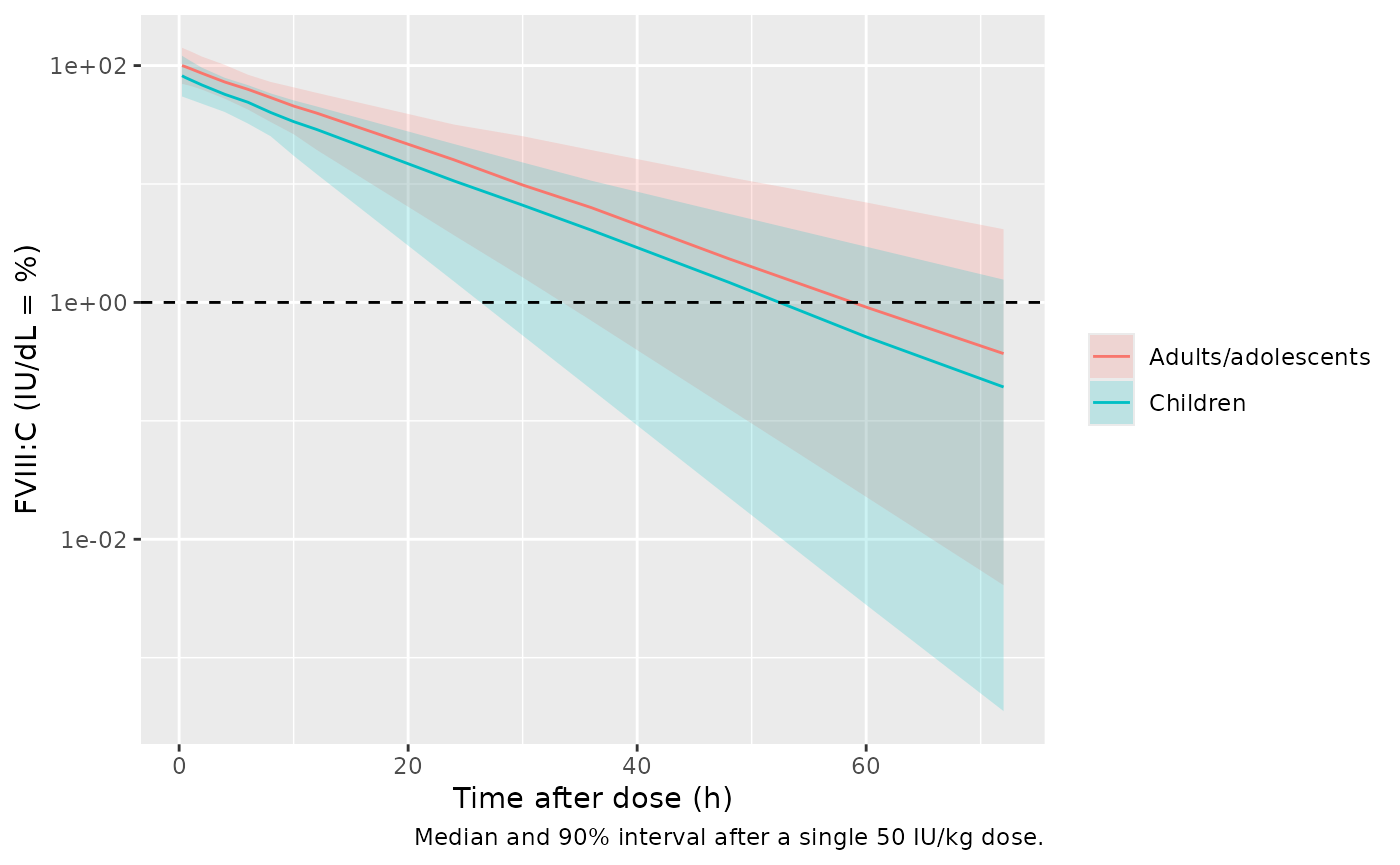
The PK sessions of the pivotal trials gave a single 50 IU/kg dose with sampling up to 48 h. The same design is simulated here (extended to 72 h for the terminal phase), and PKNCA computes the NCA parameters by age group. Tiede 2021 does not report NCA values, so there is no published comparison table; the check is internal consistency of the simulated profiles with the individual parameters.
obs_times <- c(0, 0.25, 0.5, 1, 2, 4, 6, 8, 10, 12, 24, 30, 36, 48, 60, 72)
ev_sd <- subjects |>
  rowwise() |>
  reframe(
    id = id,
    group = group,
    WT = WT,
    AGE = AGE,
    time = c(0, obs_times),
    evid = c(1L, rep(0L, length(obs_times))),
    amt = c(50 * WT, rep(0, length(obs_times))),
    cmt = "central"
  ) |>
  arrange(id, time, desc(evid))

sim_sd <- rxode2::rxSolve(
  mod,
  events = ev_sd,
  keep = "group",
  rtol = 1e-10,
  atol = 1e-12
) |>
  as.data.frame()
#> ℹ parameter labels from comments will be replaced by 'label()'

sim_sd |>
  group_by(group, time) |>
  summarise(
    Q05 = quantile(Cc, 0.05),
    Q50 = median(Cc),
    Q95 = quantile(Cc, 0.95),
    .groups = "drop"
  ) |>
  filter(time > 0) |>
  ggplot(aes(time, Q50, colour = group, fill = group)) +
  geom_ribbon(aes(ymin = Q05, ymax = Q95), alpha = 0.2, colour = NA) +
  geom_line() +
  geom_hline(yintercept = 1, linetype = "dashed") +
  scale_y_log10() +
  labs(
    x = "Time after dose (h)",
    y = "FVIII:C (IU/dL = %)",
    colour = NULL,
    fill = NULL,
    caption = "Median and 90% interval after a single 50 IU/kg dose."
  )
stopifnot(all(sim_sd$Cc >= -1e-6 * max(sim_sd$Cc)))
conc_df <- sim_sd |>
  filter(!is.na(Cc)) |>
  mutate(Cc = pmax(Cc, 0)) |>
  select(id, time, Cc, group)
dose_df <- ev_sd |>
  filter(evid == 1) |>
  select(id, time, amt, group)

conc_obj <- PKNCA::PKNCAconc(conc_df, Cc ~ time | group + id)
dose_obj <- PKNCA::PKNCAdose(
  dose_df,
  amt ~ time | group + id,
  route = "intravascular"
)
intervals <- data.frame(
  start = 0,
  end = Inf,
  cmax = TRUE,
  aucinf.obs = TRUE,
  half.life = TRUE,
  cl.obs = TRUE
)
nca_res <- PKNCA::pk.nca(PKNCA::PKNCAdata(conc_obj, dose_obj, intervals = intervals))
nca_wide <- as.data.frame(nca_res$result) |>
  select(group, id, PPTESTCD, PPORRES) |>
  pivot_wider(names_from = PPTESTCD, values_from = PPORRES)

# Individual cl and half-life from the model output.
indiv <- sim_sd |>
  group_by(id) |>
  summarise(cl_model = first(cl), vc_model = first(vc), .groups = "drop")
chk <- nca_wide |>
  left_join(indiv, by = "id") |>
  mutate(
    pct_cl = 100 * (cl.obs / cl_model - 1),
    pct_thalf = 100 * (half.life / (log(2) * vc_model / cl_model) - 1)
  )
# NCA clearance and half-life agree with the individual model values;
# residual differences are the trapezoidal AUC error and the extrapolation.
stopifnot(
  abs(median(chk$pct_cl)) < 3,
  quantile(abs(chk$pct_cl), 0.9) < 6,
  abs(median(chk$pct_thalf)) < 3
)

nca_wide |>
  group_by(group) |>
  summarise(
    across(c(cmax, aucinf.obs, half.life, cl.obs), median),
    .groups = "drop"
  ) |>
  dplyr::rename(
    "Age group" = group,
    "Cmax (IU/dL)" = cmax,
    "AUCinf (IU*h/dL)" = aucinf.obs,
    "Half-life (h)" = half.life,
    "CL (dL/h)" = cl.obs
  ) |>
knitr::kable(digits = 2, caption = "Median simulated NCA after 50 IU/kg.")| Age group | Cmax (IU/dL) | AUCinf (IU*h/dL) | Half-life (h) | CL (dL/h) |
|---|---|---|---|---|
| Adults/adolescents | 102.64 | 1340.95 | 8.90 | 2.65 |
| Children | 84.64 | 961.05 | 8.21 | 1.17 |
Figure 1: predicted FVIII:C in the activity ranges
Figure 1 of Tiede 2021 shows the first week of prophylaxis for two patients dosed three times weekly with a 2-2-3 day interval pattern, with the predicted FVIII:C time divided into the ranges 0-1%, >1-5%, >5-15%, >15-50% and >50%. The patients’ weights and doses are not reported, so the figure below shows the typical 70-kg, 20-year-old patient given an illustrative 40 IU/kg on days 0, 2 and 4.
ev_fig1 <- data.frame(
  id = 1L,
  time = c(0, 48, 96, seq(0, 168, by = 0.25)),
  evid = c(rep(1L, 3), rep(0L, length(seq(0, 168, by = 0.25)))),
  amt = c(rep(40 * 70, 3), rep(0, length(seq(0, 168, by = 0.25)))),
  cmt = "central",
  WT = 70,
  AGE = 20
) |>
  arrange(time, desc(evid))
sim_fig1 <- rxode2::rxSolve(mod_typical, events = ev_fig1) |> as.data.frame()
#> ℹ omega/sigma items treated as zero: 'etalcl', 'etalvc'

ggplot(sim_fig1, aes(time / 24, Cc)) +
  geom_hline(yintercept = c(1, 5, 15, 50), linetype = "dotted", colour = "grey50") +
  geom_line() +
  scale_y_log10(breaks = c(0.1, 1, 5, 15, 50, 100)) +
  labs(
    x = "Time (days)",
    y = "Predicted FVIII:C (%)",
    caption = "Illustrative analogue of Figure 1 of Tiede 2021 (typical patient, 40 IU/kg three times weekly)."
  )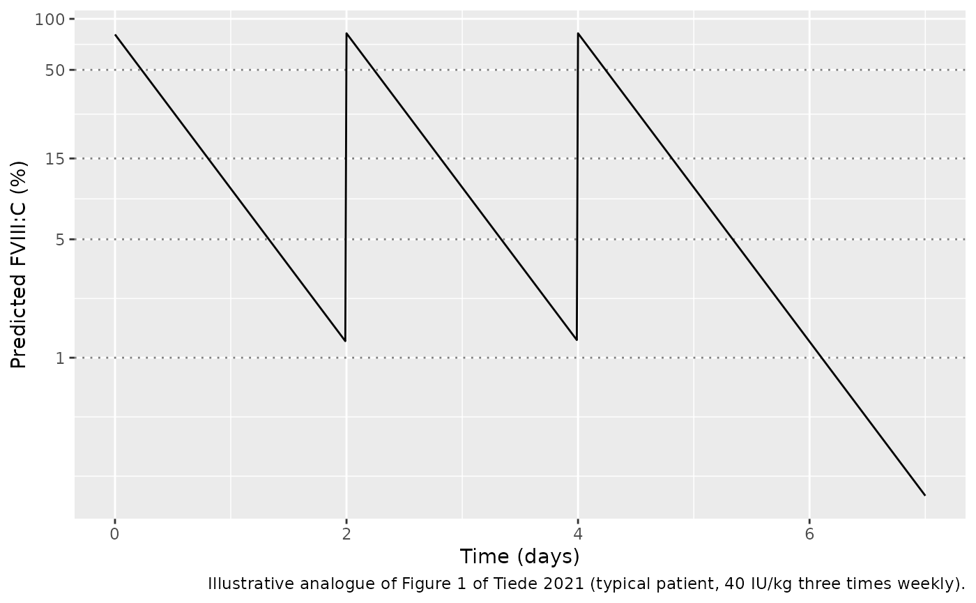
Table 3: proportion of time in each FVIII:C range
Tiede 2021 Table 3 gives the proportion of prophylaxis time spent in each predicted FVIII:C range. Those proportions were computed from each patient’s actual diary doses, which are not available. Two weeks of an illustrative three-times-weekly regimen of 40 IU/kg (days 0, 2, 4 of each week, the middle of the 20-60 IU/kg label range) are simulated for the virtual cohort, and the second week is classified into the paper’s five ranges. The comparison is a plausibility check of the model’s decay rate, not a reproduction: the dose and interval of each patient drive these proportions.
grid <- seq(168, 336, by = 0.25)
dose_times <- c(0, 48, 96, 168, 216, 264)
ev_proph <- subjects |>
  rowwise() |>
  reframe(
    id = id,
    group = group,
    WT = WT,
    AGE = AGE,
    time = c(dose_times, grid),
    evid = c(rep(1L, length(dose_times)), rep(0L, length(grid))),
    amt = c(rep(40 * WT, length(dose_times)), rep(0, length(grid))),
    cmt = "central"
  ) |>
  arrange(id, time, desc(evid))

sim_proph <- rxode2::rxSolve(mod, events = ev_proph, keep = "group") |>
  as.data.frame() |>
  filter(time < 336)

fviii_breaks <- c(-Inf, 1, 5, 15, 50, Inf)
fviii_labels <- c("0-1%", ">1-5%", ">5-15%", ">15-50%", ">50%")
time_in_range <- sim_proph |>
  mutate(range = cut(Cc, fviii_breaks, labels = fviii_labels, right = TRUE)) |>
  count(group, id, range) |>
  group_by(group, id) |>
  mutate(frac = n / sum(n)) |>
  ungroup() |>
  complete(nesting(group, id), range, fill = list(n = 0L, frac = 0))

sim_tab3 <- time_in_range |>
  group_by(group, range) |>
  summarise(simulated = round(100 * mean(frac), 1), .groups = "drop")

published_tab3 <- tibble(
  range = factor(rep(fviii_labels, 2), levels = fviii_labels),
  group = rep(c("Adults/adolescents", "Children"), each = 5),
  pivotal = c(15.58, 27.27, 25.97, 28.57, 3.90, 21.74, 26.09, 21.74, 21.74, 8.70),
  extension = c(12.85, 26.10, 25.50, 29.32, 6.22, 16.60, 26.73, 20.73, 23.04, 12.90)
)

tab3 <- sim_tab3 |>
  left_join(published_tab3, by = c("group", "range"))

# Broad plausibility bound on the 0-1% band: a 10-fold clearance or volume
# unit error drives it towards 0% or 100%. Published: 12.9-21.7%.
below1 <- time_in_range |>
  filter(range == "0-1%") |>
  group_by(group) |>
  summarise(pct = 100 * mean(frac), .groups = "drop")
stopifnot(all(below1$pct > 3), all(below1$pct < 40))

tab3 |>
  dplyr::rename(
    "Age group" = group,
    "FVIII:C range" = range,
    "Simulated, 40 IU/kg 3x weekly (%)" = simulated,
    "Table 3, pivotal (%)" = pivotal,
    "Table 3, extension (%)" = extension
  ) |>
knitr::kable(caption = "Proportion of time in each predicted FVIII:C range.")| Age group | FVIII:C range | Simulated, 40 IU/kg 3x weekly (%) | Table 3, pivotal (%) | Table 3, extension (%) |
|---|---|---|---|---|
| Adults/adolescents | 0-1% | 14.5 | 15.58 | 12.85 |
| Adults/adolescents | >1-5% | 20.8 | 27.27 | 26.10 |
| Adults/adolescents | >5-15% | 23.5 | 25.97 | 25.50 |
| Adults/adolescents | >15-50% | 28.9 | 28.57 | 29.32 |
| Adults/adolescents | >50% | 12.2 | 3.90 | 6.22 |
| Children | 0-1% | 25.0 | 21.74 | 16.60 |
| Children | >1-5% | 23.6 | 26.09 | 26.73 |
| Children | >5-15% | 20.6 | 21.74 | 20.73 |
| Children | >15-50% | 23.9 | 21.74 | 23.04 |
| Children | >50% | 6.9 | 8.70 | 12.90 |
Exposure-response: annualized bleeding rate by FVIII:C range
Tiede 2021 Table 4 reports the negative-binomial ABR of spontaneous bleeds (and spontaneous joint bleeds) in each predicted FVIII:C range, pooled over trial phases and age groups. The ABR decreases monotonically with FVIII:C. Combined with the time each simulated patient spends in each range, the Table 4 rates give an expected ABR under a given regimen. Table 5 of the paper gives the same rates split by trial phase or by age group (not crossed); the subgroup rates are much lower in the extension phase and in children at the same FVIII:C range, which the authors attribute to joint status and treatment history rather than FVIII:C.
tab4 <- tibble(
  range = factor(fviii_labels, levels = fviii_labels),
  pye = c(116.6, 214.5, 197.1, 223.7, 63.6),
  bleeds = c(303, 396, 371, 154, 13),
  joint_bleeds = c(241, 335, 337, 133, 9),
  abr_spont = c(4.16, 2.65, 2.14, 0.76, 0.21),
  abr_joint = c(3.44, 2.28, 1.99, 0.67, 0.15)
) |>
  mutate(crude_rate = bleeds / pye)

tab4 |>
  dplyr::rename(
    "FVIII:C range" = range,
    "PYE" = pye,
    "Spontaneous bleeds" = bleeds,
    "Spontaneous joint bleeds" = joint_bleeds,
    "ABR, spontaneous (NB estimate)" = abr_spont,
    "ABR, joint (NB estimate)" = abr_joint,
    "Bleeds / PYE" = crude_rate
  ) |>
knitr::kable(digits = 2, caption = "Tiede 2021 Table 4.")| FVIII:C range | PYE | Spontaneous bleeds | Spontaneous joint bleeds | ABR, spontaneous (NB estimate) | ABR, joint (NB estimate) | Bleeds / PYE |
|---|---|---|---|---|---|---|
| 0-1% | 116.6 | 303 | 241 | 4.16 | 3.44 | 2.60 |
| >1-5% | 214.5 | 396 | 335 | 2.65 | 2.28 | 1.85 |
| >5-15% | 197.1 | 371 | 337 | 2.14 | 1.99 | 1.88 |
| >15-50% | 223.7 | 154 | 133 | 0.76 | 0.67 | 0.69 |
| >50% | 63.6 | 13 | 9 | 0.21 | 0.15 | 0.20 |
expected_abr <- time_in_range |>
  left_join(tab4 |> select(range, abr_spont, abr_joint), by = "range") |>
  group_by(group, id) |>
  summarise(
    abr_spont = sum(frac * abr_spont),
    abr_joint = sum(frac * abr_joint),
    .groups = "drop"
  )

expected_abr |>
  group_by(group) |>
  summarise(
    median_abr_spont = median(abr_spont),
    median_abr_joint = median(abr_joint),
    .groups = "drop"
  ) |>
  dplyr::rename(
    "Age group" = group,
    "Expected spontaneous ABR (median)" = median_abr_spont,
    "Expected joint ABR (median)" = median_abr_joint
  ) |>
  knitr::kable(
    digits = 2,
    caption = "Expected ABR under 40 IU/kg three times weekly, using the Table 4 range-specific rates."
)| Age group | Expected spontaneous ABR (median) | Expected joint ABR (median) |
|---|---|---|
| Adults/adolescents | 1.87 | 1.63 |
| Children | 2.28 | 1.96 |
For reference, the observed overall spontaneous ABR in the trials was 1237 bleeds over 815 patient-years (1.52 per year; Table 3).
Assumptions and deviations
- Parameter source. Table 2 of Tiede 2021 cites the population PK parameters to Jimenez-Yuste 2015 (J Thromb Haemost 13:370-379). That paper was not accessible to the maintainers (publisher access blocked); all values here are as printed in Tiede 2021 Table 2 and its Results equations. Tiede 2021 describes the PK data pool as the pivotal-trial PK subgroups plus routine post-dose samples from all patients (n = 231), while the Jimenez-Yuste 2015 abstract describes 76 patients from six trials; the model is packaged as printed in Tiede 2021.
- Typical values multiply the covariate equations. The printed equations for V(W) and CL(W, A) show only the covariate factors; the Table 2 reference values (for 70 kg and 20 years) are the multipliers, as their footnotes state.
-
IIV scale. Table 2 reports inter-individual
variability as a CV (0.32 on CL, 0.22 on V) for log-normal etas; the
variances are
omega^2 = log(1 + CV^2). Reading the CV as the eta SD instead gives variances of 0.1024 and 0.0484, about 5% and 2% larger. -
Residual error. The Methods state a combined
proportional and additive residual error model but no magnitudes are
reported, so both are fixed to 0. Simulated
Ccis therefore the individual prediction, which is also what the paper’s exposure-response analysis used. - No endogenous FVIII baseline. The model follows the printed closed form with no baseline FVIII:C term; all patients had severe hemophilia A (FVIII <= 1%).
- Age and weight. The paper does not state whether age and weight were time-varying. The Table 1 values are at entry into the trial programme. Age and weight are drawn independently in the virtual cohort (their correlation within each age group is not reported).
- Exposure-response sub-model not packaged. The ABR estimates are negative-binomial regression estimates per FVIII:C category (Tables 4 and 5, Figure 2); the overdispersion and the parametric model mentioned in the Methods are not reported. They are reproduced as tables and as an expected-ABR calculation in this article rather than as a model output.
- Illustrative regimens. Figure 1 and Table 3 depend on each patient’s diary doses and intervals, which are not reported. The article uses 40 IU/kg three times weekly for both age groups; the resulting time-in-range proportions are a plausibility check only.
- Population count. The abstract states n = 187 patients (815 patient-years), while Results and Table 1 give 231 patients (168 + 63). The model metadata uses 231.
- No erratum or correction to Tiede 2021 was found (checked 2026-09-28).