Apramycin translational PKPD in complicated urinary tract infection (Hernandez-Lozano 2025)

Model and source

This paper contributed three model files, matching the three analysis layers the authors built in sequence: an in vitro time-kill fit, a mouse in vivo pharmacokinetic-pharmacodynamic (PKPD) model that re-estimates the same pharmacodynamic structure on kidney and bladder colony counts, and a human prediction that keeps that pharmacodynamic component and swaps in a published human population pharmacokinetic model.

mod_invitro <- rxode2::rxode(readModelDb("HernandezLozano_2025_apramycin_invitro"))
mod_mouse   <- rxode2::rxode(readModelDb("HernandezLozano_2025_apramycin_mouse"))
mod_human   <- rxode2::rxode(readModelDb("HernandezLozano_2025_apramycin_human"))
#> ℹ parameter labels from comments will be replaced by 'label()'

• Citation: Hernandez-Lozano I, Aranzana-Climent V, Cao S, Matias C, Hansen JU, Liepinsh E, Hughes D, Hobbie SN, Vingsbo Lundberg C, Friberg LE. Model-informed drug development for antimicrobials: translational pharmacokinetic-pharmacodynamic modelling of apramycin to facilitate prediction of efficacious dose in complicated urinary tract infections. J Antimicrob Chemother. 2025 Feb 3;80(2):302-311. doi:10.1093/jac/dkae409. PMID: 39545353. PMCID: PMC11695905. In vitro PD structure: Materials and methods, ‘PKPD modelling’, plus the schematic in Figure 1. Parameter estimates and 95% CIs: Table 1, section ‘In vitro PD parameters’. MIC values: Results, ‘In vitro time-kill curves and PD modelling’. The natural bacterial death rate kd was fixed to 0.179 per hour from Nielsen EI, Cars O, Friberg LE, Antimicrob Agents Chemother 2011;55:4619-30 (doi:10.1128/AAC.00182-11).
• Article: https://doi.org/10.1093/jac/dkae409
• PubMed Central open-access copy: https://pmc.ncbi.nlm.nih.gov/articles/PMC11695905/
• Upstream mouse population PK (Sou 2021): https://doi.org/10.1002/cpt.2104
• Upstream human population PK (Zhao 2022): https://doi.org/10.1093/jac/dkac225

Model file	Role
HernandezLozano_2025_apramycin_invitro	Static time-kill fit for two Escherichia coli strains at pH 7.4 and pH 6
HernandezLozano_2025_apramycin_mouse	Mouse complicated urinary tract infection (cUTI) PKPD: subcutaneous PK driving kidney and bladder colony counts
HernandezLozano_2025_apramycin_human	Human efficacy prediction: the Zhao 2022 population PK driving the same kidney and bladder pharmacodynamics

Structure

Both organs and the in vitro system share one bacterial structure (source Figure 1). Two subpopulations, a main apramycin-susceptible one (1) and one with decreased susceptibility (2), each carry a growing drug-susceptible state S and a dormant drug-insusceptible state D:

• growth of S at kg (reduced by Redukg percent in subpopulation 2);
• natural death of both states at kd;
• density-dependent transfer S -> D at ksr = (kg - kd) * Btot / Bmax, which drives the total count to Bmax at stationary phase; no back transfer;
• apramycin adds to the death rate of the S states only, through a power model normalized to the MIC, kdrug = Slope * (Cu/MIC)^gamma with gamma fixed to 1;
• apramycin drives the transfer of bacteria from subpopulation 1 to subpopulation 2 at rate kada * (Cu/MIC), so the inoculum contains no pre-existing resistant fraction.

In vivo the kidney is assumed to be at pH 7.4 and the bladder at pH 6, so each organ normalizes the unbound plasma concentration by the MIC measured at its own pH.

Population

The in vitro layer used two Escherichia coli urinary isolates, EN591 (an MDR rmtB isolate) and ATCC 700336 / EN1085 (a trimethoprim/sulfamethoxazole resistant isolate), in static time-kill experiments in pH-buffered Mueller-Hinton II broth at 0.25 to 8 x MIC, sampled to 28 h.

The in vivo layer used 286 female C3H/HeJ mice, 6 weeks old, mean weight 16.8 g (range 12.3 to 21.2 g), across three studies (source Supplementary Table S1). Ascending cUTI was established by transurethral inoculation of the bladder; animals were immunocompetent and received 5% glucose in the drinking water to induce diuresis. Apramycin was given subcutaneously twice daily at 24, 30, 48, 54, 72 and 78 h after inoculation, and kidneys and bladder were harvested for colony counts at 6, 10, 24, 30, 48, 72 and 96 h after inoculation.

The human layer is a simulation, not a fitted population: a typical 75 kg adult with a renal function of 120 mL/min receiving single 30 min intravenous infusions at the five dose levels of the apramycin Phase I trial. The underlying population PK model was developed by Zhao 2022 in 30 healthy volunteers (480 plasma and 179 urine observations).

str(mod_mouse$population, max.level = 1)
#> List of 10
#>  $ species       : chr "mouse (C3H/HeJ, female, 6 weeks old)"
#>  $ n_subjects    : int 286
#>  $ n_studies     : int 3
#>  $ weight_range  : chr "12.3-21.2 g"
#>  $ weight_median : chr "16.8 g (mean)"
#>  $ sex_female_pct: num 100
#>  $ disease_state : chr "Complicated urinary tract infection (ascending cUTI) established by transurethral inoculation of 5x10^7 CFU of "| __truncated__
#>  $ dose_range    : chr "Apramycin 1.5-30 mg/kg subcutaneously twice daily in the primary studies (3, 10 and 30 mg/kg for EN591; 1.5, 5 "| __truncated__
#>  $ regions       : chr "Statens Serum Institut, Denmark (Studies 1 and 2); Pharmacology Discovery Services Taiwan (Study 3)"
#>  $ notes         : chr "Animal counts by strain, dose and sampling time are in Supplementary Table S1: 286 mice in total across three s"| __truncated__

Source trace

Every ini() entry carries an in-file comment naming its source location. The tables below collect them for review.

Shared pharmacodynamic structure

Equation	Source location
Two subpopulations x two states (S, D), drug on S only	Figure 1; Materials and methods, “PKPD modelling”
ksr = (kg - kd) * Btot / Bmax	Figure 1 (ksr “as a response to high population densities”); the Nielsen-lineage form used by the cited framework
kdrug = Slope * (Cu/MIC)^gamma	Materials and methods: drug “increasing the death rate in the S state by a rate kdrug … modelled by a power model”; Table 1 Slope rows are “normalized by MIC”; Table 1 gamma = 1 FIX
S1 -> S2 at kada * (Cu/MIC)	Materials and methods: “A rate constant (kada), describing the drug-driven transfer from the susceptible to the resistant population, was included in the model rather than assuming initial pre-existing percentages of each subpopulation”
kg2 = kg1 * (1 - Redukg/100)	Table 1 Redukg rows, unit column “%”
Kidney at pH 7.4, bladder at pH 6	Discussion: “The concentration in the central compartment was normalized to the in vitro MIC assuming pH 7.4 and pH 6 for the kidneys and bladder, respectively”

HernandezLozano_2025_apramycin_invitro

Parameter	Value	Source location
lkgEn591, lkgAtcc	1.64, 2.27 /h	Table 1, in vitro kg
redukg	0.63 %	Table 1, in vitro Redukg
lkd	0.179 /h FIXED	Table 1, in vitro kd; Methods cite Nielsen 2011 (reference 23)
lbmax	9.18 log10 CFU/mL	Table 1, in vitro Bmax
linoc	5.53 log10 CFU/mL	Table 1, in vitro Inoc
gam	1 FIXED	Table 1, in vitro gamma
slopeSEn591ph6/ph74, slopeSAtcc	1.31, 2.37, 2.99 /h	Table 1, in vitro SlopeS
slopeREn591ph6/ph74, slopeRAtcc	0.385, 0.254, 0.776 /h	Table 1, in vitro SlopeR
kadaEn591ph6/ph74, kadaAtcc	0.080/1000, 0.028/1000, 0.210/1000 /h	Table 1, in vitro row kada x 1000
micEn591ph74, micEn591ph6, micAtccph74, micAtccph6	8, 32, 4, 16 mg/L, all FIXED	Results, “In vitro time-kill curves and PD modelling”
Selection of the parameter set on BACT x PH_MEDIUM	–	Results: for ATCC 700336 “the same parameters” describe both pH levels, whereas for EN591 “differences in bacterial regrowth at 4 x MIC between pH 6 and pH 7.4 conditions resulted in different drug effect parameters”
addSd	0 FIXED	Methods state an additive residual error model; no value is reported (see Errata)

HernandezLozano_2025_apramycin_mouse

Parameter	Value	Source location
lcl, lvc	8.49 L/h/70 kg, 6.55 L/70 kg, both FIXED	Sou 2021 Table 1, mouse column
lka30, powka	2.17 /h, -0.160, both FIXED	Sou 2021 Table 1 mouse column; Eq. 3 ka = ka30 * (Dose/30)^pow
e_wt_cl, e_wt_vc	0.75, 1, both FIXED	Sou 2021 Eqs. 1-2
lfdepot	log(1) FIXED	Sou 2021: F set to 1 for the subcutaneous-only species
fu	0.916 FIXED	Methods, “PKPD modelling”: unbound fraction in mouse plasma 91.6%
micEn591ph74/ph6, micAtccph74/ph6	8, 32, 4, 16 mg/L, all FIXED	Results, “In vitro time-kill curves and PD modelling”
lkg1kEn591, lkg1kAtcc	0.694, 0.205 /h	Table 1, in vivo kg1k
redukgkEn591, redukgkAtcc	25.4, 6.9 %	Table 1, in vivo Reduckgk
lkdkEn591, lkdkAtcc	0.526 /h; 0.179 /h FIXED	Table 1, in vivo kd,k
slopeSk, slopeRk, kadak	9.05, 0.066, 0.031 /h	Table 1, in vivo SlopeSk, SlopeRk, kada,k
lbmaxk, linock	6.49 FIXED, 5.70 log10 CFU/organ	Table 1, in vivo Bmax,k, Inock
lkg1bEn591, lkg1bAtcc	1.51, 0.228 /h	Table 1, in vivo kg1b
redukgbEn591, redukgbAtcc	25.2, 6.9 %	Table 1, in vivo Reduckgb
lkdbEn591, lkdbAtcc	1.16 /h; 0.179 /h FIXED	Table 1, in vivo kd,b
slopeSb, slopeRb, kadab	191, 0.276, 1.35 /h	Table 1, in vivo SlopeSb, SlopeRb, kada,b
lbmaxb, linocb	7.07 FIXED, 4.42 log10 CFU/organ	Table 1, in vivo Bmax,b, Inocb
gam	1 FIXED	Table 1, in vivo gamma
propSd	0.49 FIXED	Sou 2021 Table 1, mouse ERR = 49%
addSd_cfuKidney, addSd_cfuBladder	0 FIXED	Methods state an additive residual error model; no value is reported (see Errata)

HernandezLozano_2025_apramycin_human

Parameter	Value	Source location
lcl	5.54 L/h FIXED	Zhao 2022 Table 2, plasma+urine column, CL
lvc, lq, lvp, lq2, lvp2, lq3, lvp3	8.61 L, 0.127 L/h, 2.29 L, 13.6 L/h, 2.81 L, 1.01 L/h, 2.38 L, all FIXED	Zhao 2022 Table 2, plasma+urine column, Vc, Q2, V2, Q3, V3, Q4, V4
fe	0.900 FIXED	Zhao 2022 Table 2, plasma+urine column, Fe
crclRef, e_wt_cl, e_wt_vc	124 mL/min, 0.75, 1, all FIXED	Zhao 2022 Table 2 footnote a and Methods
fu	0.929 FIXED	Methods, “Prediction of human efficacy”: unbound fraction 92.9%
etalcl + etalvc + etalvp2 block	0.0205237 / 0.0240203 / 0.1039655 / -0.0323211 / -0.1673124 / 0.3181215	Zhao 2022 Table 2: IIV CV 14.4%, 33.1%, 61.2% converted with omega^2 = log(CV^2 + 1); correlations 0.52, -0.40, -0.92 (footnote d)
etalvp3	0.0191367	Zhao 2022 Table 2: IIV in V4 13.9% CV
propSd	0.0879 FIXED	Zhao 2022 Table 2, plasma+urine column, Prop plasma = 8.79%
linock, linocb	10^6, 10^5 CFU/organ, both FIXED	Methods, “Prediction of human efficacy”
Remaining pharmacodynamic parameters	as in the mouse file	Table 1, in vivo section

Simulation helpers

# rxSolve() drops IIV only when the model has etas to drop; zeroRe() warns on a
# model with none (see known-vignette-failure-patterns.md pattern 9).
solve_typical <- function(mod, ev, ...) {
  ui <- rxode2::rxode(mod)
  if (any(!is.na(ui$iniDf$neta1))) {
    as.data.frame(rxode2::rxSolve(rxode2::zeroRe(mod), ev, useLinCmt = FALSE, ...))
  } else {
    as.data.frame(rxode2::rxSolve(mod, ev, useLinCmt = FALSE, ...))
  }
}

# Value of `col` at (or nearest to) time `t`; errors rather than returning NA.
at_time <- function(d, t, col) {
  i <- which.min(abs(d$time - t))
  stopifnot(length(i) == 1L, abs(d$time[i] - t) < 1e-6)
  d[[col]][i]
}

In vitro time-kill (replicates Figure 2)

Observation rows point at the ODE state bact_s1; rxode2 returns the algebraic observable Cc (here the log10 total count) as a column regardless.

# `mic` here is only the design quantity used to convert a multiple of the MIC
# into a bath concentration; the model derives the MIC it uses internally from
# BACT and PH_MEDIUM, so the two must agree by construction.
invitro_conditions <- tibble::tribble(
  ~condition,            ~BACT, ~PH_MEDIUM, ~mic,
  "EN591, pH 6",           591,        6.0,   32,
  "EN591, pH 7.4",         591,        7.4,    8,
  "ATCC 700336, pH 6",  700336,        6.0,   16,
  "ATCC 700336, pH 7.4",700336,        7.4,    4
)
xmic_levels <- c(0, 0.25, 0.5, 1, 2, 4, 8)

sim_invitro <- purrr::pmap_dfr(invitro_conditions, function(condition, BACT, PH_MEDIUM, mic) {
  purrr::map_dfr(xmic_levels, function(xmic) {
    ev <- dplyr::bind_rows(
      data.frame(time = 0, amt = xmic * mic, evid = 1L,
                 cmt = "apramycin", dvid = NA_integer_),
      data.frame(time = seq(0, 28, by = 0.1), amt = NA_real_, evid = 0L,
                 cmt = "bact_s1", dvid = 1L)
    ) |>
      dplyr::arrange(time, dplyr::desc(evid)) |>
      dplyr::mutate(id = 1L, BACT = BACT, PH_MEDIUM = PH_MEDIUM)
    solve_typical(mod_invitro, ev) |>
      dplyr::transmute(time, logcfu = Cc,
                       condition = condition,
                       xmic = factor(xmic, levels = xmic_levels,
                                     labels = paste0(xmic_levels, " x MIC")))
  })
})

ggplot(sim_invitro, aes(time, logcfu)) +
  geom_line(linewidth = 0.6) +
  facet_grid(condition ~ xmic) +
  coord_cartesian(ylim = c(-1, 10)) +
  labs(x = "Time (h)", y = "Bacterial count (log10 CFU/mL)") +
  theme_bw(base_size = 9)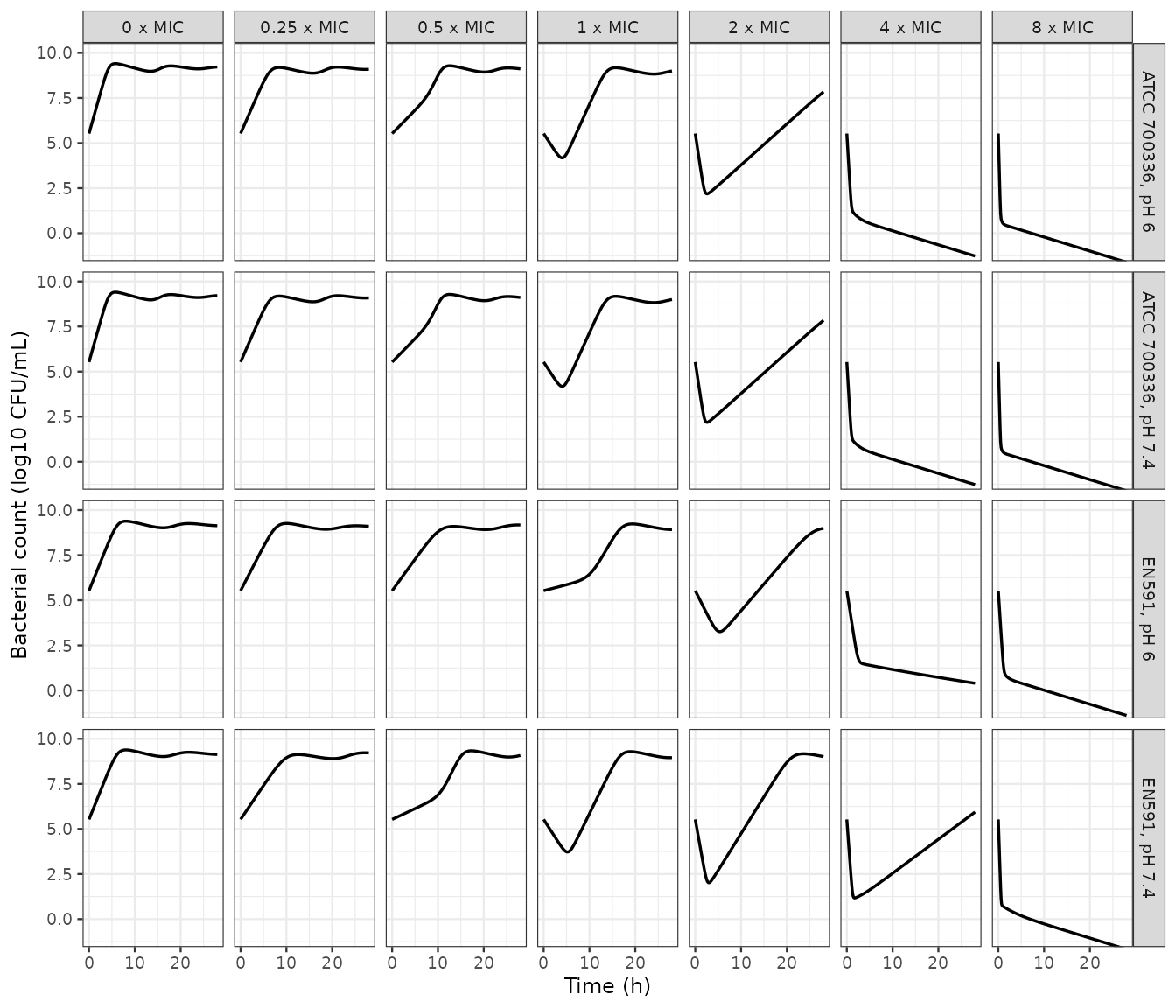

Replicates Figure 2 of Hernandez-Lozano 2025: model-predicted in vitro time-kill curves for the two strains at pH 6 and pH 7.4.

Two features of Figure 2 are structural signatures worth asserting rather than eyeballing. First, the growth control must plateau at Bmax. Second, the paper gives the EN591 pH-6 versus pH-7.4 difference at 4 x MIC as its stated reason for keeping separate drug-effect parameters for that strain: at pH 7.4 the culture regrows after the initial kill, at pH 6 it does not.

end28 <- sim_invitro |>
  dplyr::filter(abs(time - 28) < 1e-6) |>
  dplyr::select(condition, xmic, logcfu)

bmax_log10 <- log10(exp(mod_invitro$theta[["lbmax"]]))
control_end <- end28$logcfu[end28$xmic == "0 x MIC"]
stopifnot(length(control_end) == 4L, all(abs(control_end - bmax_log10) < 0.1))

nadir <- sim_invitro |>
  dplyr::group_by(condition, xmic) |>
  dplyr::summarise(nadir = min(logcfu), final = dplyr::last(logcfu), .groups = "drop") |>
  dplyr::mutate(regrowth = final - nadir)

get_regrowth <- function(cond, xm) {
  v <- nadir$regrowth[nadir$condition == cond & nadir$xmic == xm]
  if (length(v) != 1L) stop("no unique row for ", cond, " at ", xm)
  v
}
# EN591 at 4 x MIC: substantial regrowth at pH 7.4, essentially none at pH 6.
stopifnot(get_regrowth("EN591, pH 7.4", "4 x MIC") > 4)
stopifnot(get_regrowth("EN591, pH 6",   "4 x MIC") < 0.1)
# ATCC 700336 shares one MIC-normalized parameter set across pH, so the two
# pH panels must be numerically identical.
atcc <- end28 |> dplyr::filter(grepl("ATCC", condition)) |>
  tidyr::pivot_wider(names_from = condition, values_from = logcfu)
stopifnot(nrow(atcc) == length(xmic_levels),
          max(abs(atcc$`ATCC 700336, pH 6` - atcc$`ATCC 700336, pH 7.4`)) < 1e-8)

end28 |>
  tidyr::pivot_wider(names_from = xmic, values_from = logcfu) |>
  dplyr::rename("Condition" = condition) |>
  knitr::kable(digits = 2,
               caption = "Model-predicted log10 CFU/mL at 28 h (compare Figure 2).")

Model-predicted log10 CFU/mL at 28 h (compare Figure 2).

Condition	0 x MIC	0.25 x MIC	0.5 x MIC	1 x MIC	2 x MIC	4 x MIC	8 x MIC
EN591, pH 6	9.13	9.10	9.17	8.92	8.98	0.40	-1.38
EN591, pH 7.4	9.13	9.22	9.08	8.96	9.01	5.94	-1.67
ATCC 700336, pH 6	9.22	9.09	9.11	9.00	7.84	-1.27	-1.61
ATCC 700336, pH 7.4	9.22	9.09	9.11	9.00	7.84	-1.27	-1.61

Mouse cUTI (replicates Figure 3)

Model time zero is 6 h after bacterial inoculation, the first sampling time and the point at which Inoc_k and Inoc_b were estimated. Doses therefore fall at model times 18, 24, 42, 48, 66 and 72 h.

wt_mouse <- 0.0168               # mean weight, Supplementary methods
dose_times <- c(18, 24, 42, 48, 66, 72)

mouse_arms <- tibble::tribble(
  ~strain,        ~BACT,   ~mgkg,
  "EN591",           591,      0,
  "EN591",           591,      3,
  "EN591",           591,     10,
  "EN591",           591,     30,
  "ATCC 700336",  700336,      0,
  "ATCC 700336",  700336,    1.5,
  "ATCC 700336",  700336,      5,
  "ATCC 700336",  700336,     15
)

sim_mouse <- purrr::pmap_dfr(mouse_arms, function(strain, BACT, mgkg) {
  obs <- data.frame(time = seq(0, 90, by = 0.25), amt = NA_real_, evid = 0L,
                    cmt = "central", dvid = 1L)
  ev <- if (mgkg > 0) {
    dplyr::bind_rows(
      data.frame(time = dose_times, amt = mgkg * wt_mouse, evid = 1L,
                 cmt = "depot", dvid = NA_integer_),
      obs
    )
  } else {
    obs
  }
  ev <- ev |>
    dplyr::arrange(time, dplyr::desc(evid)) |>
    dplyr::mutate(
      id = 1L, WT = wt_mouse, BACT = BACT,
      # With no dose event the absorption rate constant is unused, but it must
      # still be finite: Sou 2021 Eq. 3 raises the dose level to a negative
      # power, so a zero dose level would give an infinite ka.
      DOSE_APRAMYCIN_MGKG = if (mgkg > 0) mgkg else 30
    )
  solve_typical(mod_mouse, ev) |>
    dplyr::transmute(
      time_pi = time + 6,        # hours after bacterial inoculation
      Kidney = cfuKidney, Bladder = cfuBladder,
      strain = strain,
      arm = paste0(mgkg, " mg/kg")
    )
})

sim_mouse_long <- sim_mouse |>
  tidyr::pivot_longer(c(Kidney, Bladder), names_to = "organ", values_to = "logcfu") |>
  dplyr::mutate(
    organ = factor(organ, levels = c("Kidney", "Bladder")),
    arm = factor(arm, levels = c("0 mg/kg", "1.5 mg/kg", "3 mg/kg", "5 mg/kg",
                                 "10 mg/kg", "15 mg/kg", "30 mg/kg"))
  )

ggplot(sim_mouse_long, aes(time_pi, logcfu)) +
  geom_line(linewidth = 0.6) +
  facet_grid(strain + organ ~ arm) +
  scale_x_continuous(breaks = c(0, 24, 48, 72, 96)) +
  coord_cartesian(ylim = c(0, 10)) +
  labs(x = "Time after inoculation (h)", y = "Bacterial load (log10 CFU/organ)") +
  theme_bw(base_size = 9)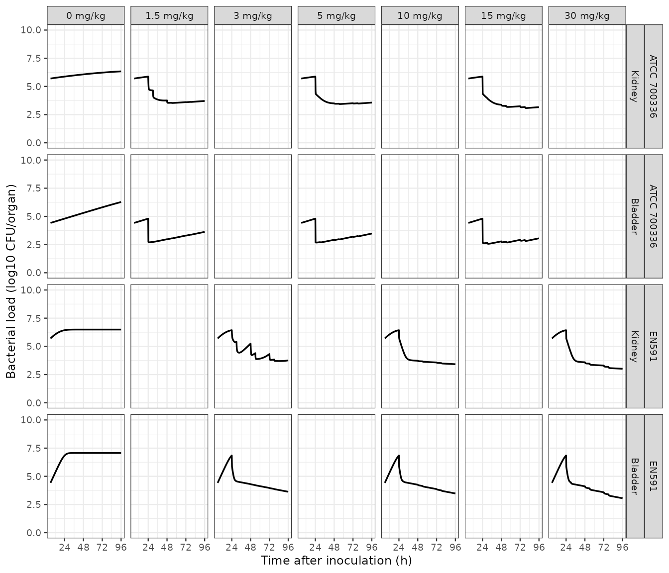

Replicates Figure 3 of Hernandez-Lozano 2025: typical-value bacterial burden in mouse kidneys and bladder after twice-daily subcutaneous apramycin, EN591 (upper) and ATCC 700336 (lower).

The paper’s quantitative in vivo claims are that the untreated control plateaus at the fixed Bmax of each organ, and that at 96 h after inoculation (72 h after the start of treatment) burden is “reduced by at least 2-log in comparison with the start of treatment (24 h after inoculation) and with respect to vehicle control”.

pick <- function(strain_, arm_, organ_, t_) {
  v <- sim_mouse_long$logcfu[sim_mouse_long$strain == strain_ &
                               sim_mouse_long$arm == arm_ &
                               sim_mouse_long$organ == organ_ &
                               abs(sim_mouse_long$time_pi - t_) < 1e-6]
  if (length(v) != 1L) stop("no unique row for ", strain_, " ", arm_, " ", organ_, " at ", t_, " h")
  v
}

bmax_kidney <- log10(exp(mod_mouse$theta[["lbmaxk"]]))
bmax_bladder <- log10(exp(mod_mouse$theta[["lbmaxb"]]))
# EN591 grows fast enough to be at Bmax by 96 h in both organs.
stopifnot(abs(pick("EN591", "0 mg/kg", "Kidney", 96) - bmax_kidney) < 0.02)
stopifnot(abs(pick("EN591", "0 mg/kg", "Bladder", 96) - bmax_bladder) < 0.02)
# ATCC 700336 grows about 7-fold more slowly and has not yet reached Bmax, but
# is still approaching it monotonically.
stopifnot(pick("ATCC 700336", "0 mg/kg", "Kidney", 96) < bmax_kidney,
          pick("ATCC 700336", "0 mg/kg", "Kidney", 96) >
            pick("ATCC 700336", "0 mg/kg", "Kidney", 24))

mouse_reduction <- purrr::pmap_dfr(
  dplyr::filter(mouse_arms, mgkg > 0),
  function(strain, BACT, mgkg) {
    arm_ <- paste0(mgkg, " mg/kg")
    purrr::map_dfr(c("Kidney", "Bladder"), function(org) {
      tibble::tibble(
        Strain = strain, Arm = arm_, Organ = org,
        `Start of treatment (24 h)` = pick(strain, arm_, org, 24),
        `End of treatment (96 h)` = pick(strain, arm_, org, 96),
        `Change vs start` = pick(strain, arm_, org, 96) - pick(strain, arm_, org, 24),
        `Change vs control` = pick(strain, arm_, org, 96) -
          pick(strain, "0 mg/kg", org, 96)
      )
    })
  }
)

stopifnot(nrow(mouse_reduction) == 12L)
# The EN591 arms are the ones the >=2-log sentence in Results refers to.
en591_red <- dplyr::filter(mouse_reduction, Strain == "EN591")
stopifnot(nrow(en591_red) == 6L,
          all(en591_red$`Change vs start` <= -2),
          all(en591_red$`Change vs control` <= -2))
# Every arm of both strains clears at least 2 log relative to its own control.
stopifnot(all(mouse_reduction$`Change vs control` <= -2))
# Dose-ordering: within each strain and organ, the 96 h burden falls with dose.
stopifnot(
  mouse_reduction |>
    dplyr::group_by(Strain, Organ) |>
    dplyr::summarise(mono = !is.unsorted(rev(`End of treatment (96 h)`)),
                     .groups = "drop") |>
    dplyr::pull(mono) |>
    all()
)

knitr::kable(mouse_reduction, digits = 2,
             caption = "Model-predicted log10 CFU/organ at the end of treatment (compare Figure 3).")

Model-predicted log10 CFU/organ at the end of treatment (compare Figure 3).

Strain	Arm	Organ	Start of treatment (24 h)	End of treatment (96 h)	Change vs start	Change vs control
EN591	3 mg/kg	Kidney	6.43	3.76	-2.67	-2.73
EN591	3 mg/kg	Bladder	6.85	3.63	-3.22	-3.44
EN591	10 mg/kg	Kidney	6.43	3.42	-3.02	-3.07
EN591	10 mg/kg	Bladder	6.85	3.48	-3.37	-3.59
EN591	30 mg/kg	Kidney	6.43	3.01	-3.42	-3.48
EN591	30 mg/kg	Bladder	6.85	3.05	-3.79	-4.02
ATCC 700336	1.5 mg/kg	Kidney	5.87	3.71	-2.16	-2.63
ATCC 700336	1.5 mg/kg	Bladder	4.80	3.63	-1.18	-2.65
ATCC 700336	5 mg/kg	Kidney	5.87	3.57	-2.31	-2.77
ATCC 700336	5 mg/kg	Bladder	4.80	3.48	-1.32	-2.80
ATCC 700336	15 mg/kg	Kidney	5.87	3.16	-2.71	-3.17
ATCC 700336	15 mg/kg	Bladder	4.80	3.06	-1.75	-3.22

In vitro to in vivo translation

Two headline numbers of the abstract are pure parameter identities and can be recomputed exactly from the packaged ini() values: a 76% to 98% reduction of bacterial net growth, and a 3- to 145-fold increase in apramycin potency in vivo relative to in vitro. Net growth is knet = kg - kd. Potency is compared at matched pH: kidney against the in vitro pH-7.4 parameters and bladder against pH 6.

th_iv <- mod_invitro$theta
th_mo <- mod_mouse$theta

knet <- function(kg, kd) kg - kd
kd_invitro <- exp(th_iv[["lkd"]])

translation <- tibble::tribble(
  ~Strain,        ~Organ,   ~knet_invitro, ~knet_invivo, ~slope_invitro, ~slope_invivo,
  "EN591",       "Kidney",
    knet(exp(th_iv[["lkgEn591"]]), kd_invitro),
    knet(exp(th_mo[["lkg1kEn591"]]), exp(th_mo[["lkdkEn591"]])),
    th_iv[["slopeSEn591ph74"]], th_mo[["slopeSk"]],
  "EN591",       "Bladder",
    knet(exp(th_iv[["lkgEn591"]]), kd_invitro),
    knet(exp(th_mo[["lkg1bEn591"]]), exp(th_mo[["lkdbEn591"]])),
    th_iv[["slopeSEn591ph6"]], th_mo[["slopeSb"]],
  "ATCC 700336", "Kidney",
    knet(exp(th_iv[["lkgAtcc"]]), kd_invitro),
    knet(exp(th_mo[["lkg1kAtcc"]]), exp(th_mo[["lkdkAtcc"]])),
    th_iv[["slopeSAtcc"]], th_mo[["slopeSk"]],
  "ATCC 700336", "Bladder",
    knet(exp(th_iv[["lkgAtcc"]]), kd_invitro),
    knet(exp(th_mo[["lkg1bAtcc"]]), exp(th_mo[["lkdbAtcc"]])),
    th_iv[["slopeSAtcc"]], th_mo[["slopeSb"]]
) |>
  dplyr::mutate(
    `Net-growth reduction (%)` = 100 * (1 - knet_invivo / knet_invitro),
    `Potency increase (fold)` = slope_invivo / slope_invitro
  )

# Abstract: "76%-98% reduction of bacterial net growth".
stopifnot(round(min(translation$`Net-growth reduction (%)`)) == 76,
          round(max(translation$`Net-growth reduction (%)`)) == 98 |
            round(max(translation$`Net-growth reduction (%)`)) == 99)
# Abstract: "3- to 145-fold increase in apramycin potency".
stopifnot(round(min(translation$`Potency increase (fold)`)) == 3,
          round(max(translation$`Potency increase (fold)`)) == 146 |
            round(max(translation$`Potency increase (fold)`)) == 145)

translation |>
  dplyr::select(Strain, Organ,
                "knet in vitro (1/h)" = knet_invitro,
                "knet in vivo (1/h)" = knet_invivo,
                `Net-growth reduction (%)`,
                "SlopeS in vitro (1/h)" = slope_invitro,
                "SlopeS in vivo (1/h)" = slope_invivo,
                `Potency increase (fold)`) |>
  knitr::kable(digits = c(0, 0, 3, 3, 0, 2, 2, 1),
               caption = "In vitro to in vivo translation, recomputed from the packaged parameters. The abstract reports 76%-98% net-growth reduction and a 3- to 145-fold potency increase.")

In vitro to in vivo translation, recomputed from the packaged parameters. The abstract reports 76%-98% net-growth reduction and a 3- to 145-fold potency increase.

Strain	Organ	knet in vitro (1/h)	knet in vivo (1/h)	Net-growth reduction (%)	SlopeS in vitro (1/h)	SlopeS in vivo (1/h)	Potency increase (fold)
EN591	Kidney	1.461	0.168	89	2.37	9.05	3.8
EN591	Bladder	1.461	0.350	76	1.31	191.00	145.8
ATCC 700336	Kidney	2.091	0.026	99	2.99	9.05	3.0
ATCC 700336	Bladder	2.091	0.049	98	2.99	191.00	63.9

en591_reduction <- translation[["Net-growth reduction (%)"]][translation$Strain == "EN591"]
en591_kidney_pct <- sprintf("%.1f%%", max(en591_reduction))
en591_bladder_pct <- sprintf("%.1f%%", min(en591_reduction))

The one number that does not recompute exactly is the Discussion’s “up to 91%” net-growth reduction for EN591: the largest EN591 value here is 88.5%, in the kidney. The abstract’s own range, 76% to 98%, is consistent with the table. This is recorded in the Errata below.

Human efficacy prediction (replicates Figure 5)

wt_human <- 75
crcl_human <- 120
human_doses <- c(0.3, 1.2, 3.6, 10.8, 30)

human_events <- function(mgkg, bact, wt = wt_human, crcl = crcl_human,
                         times = seq(0, 48, by = 0.1)) {
  amt_mg <- mgkg * wt
  dplyr::bind_rows(
    data.frame(time = 0, amt = amt_mg, rate = amt_mg / 0.5, evid = 1L,
               cmt = "central", dvid = NA_integer_),
    data.frame(time = times, amt = NA_real_, rate = NA_real_, evid = 0L,
               cmt = "central", dvid = 1L)
  ) |>
    dplyr::arrange(time, dplyr::desc(evid)) |>
    dplyr::mutate(id = 1L, WT = wt, CRCL = crcl, BACT = bact)
}

sim_human <- tidyr::expand_grid(
  tibble::tibble(strain = c("EN591", "ATCC700336"), BACT = c(591, 700336)),
  mgkg = human_doses
) |>
  purrr::pmap_dfr(function(strain, BACT, mgkg) {
    solve_typical(mod_human, human_events(mgkg, BACT)) |>
      dplyr::transmute(time, Kidney = cfuKidney, Bladder = cfuBladder,
                       strain = strain,
                       arm = factor(paste0(mgkg, " mg/kg"),
                                    levels = paste0(human_doses, " mg/kg")))
  }) |>
  tidyr::pivot_longer(c(Kidney, Bladder), names_to = "organ", values_to = "logcfu") |>
  dplyr::mutate(organ = factor(organ, levels = c("Kidney", "Bladder")))
#> ℹ omega/sigma items treated as zero: 'etalcl', 'etalvc', 'etalvp2', 'etalvp3'
#> ℹ omega/sigma items treated as zero: 'etalcl', 'etalvc', 'etalvp2', 'etalvp3'
#> ℹ omega/sigma items treated as zero: 'etalcl', 'etalvc', 'etalvp2', 'etalvp3'
#> ℹ omega/sigma items treated as zero: 'etalcl', 'etalvc', 'etalvp2', 'etalvp3'
#> ℹ omega/sigma items treated as zero: 'etalcl', 'etalvc', 'etalvp2', 'etalvp3'
#> ℹ omega/sigma items treated as zero: 'etalcl', 'etalvc', 'etalvp2', 'etalvp3'
#> ℹ omega/sigma items treated as zero: 'etalcl', 'etalvc', 'etalvp2', 'etalvp3'
#> ℹ omega/sigma items treated as zero: 'etalcl', 'etalvc', 'etalvp2', 'etalvp3'
#> ℹ omega/sigma items treated as zero: 'etalcl', 'etalvc', 'etalvp2', 'etalvp3'
#> ℹ omega/sigma items treated as zero: 'etalcl', 'etalvc', 'etalvp2', 'etalvp3'

ggplot(sim_human, aes(time, logcfu)) +
  geom_line(linewidth = 0.6) +
  facet_grid(strain + organ ~ arm) +
  scale_x_continuous(breaks = c(0, 12, 24, 36, 48)) +
  coord_cartesian(ylim = c(0, 10)) +
  labs(x = "Time after dose (h)", y = "Bacterial load (log10 CFU/organ)") +
  theme_bw(base_size = 9)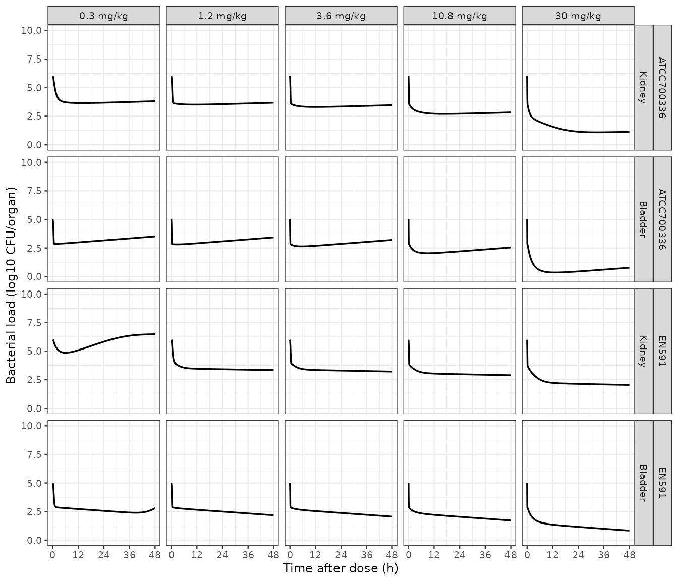

Replicates Figure 5 of Hernandez-Lozano 2025: predicted bacterial load in human kidneys and bladder over 48 h after a single 30 min intravenous infusion of apramycin, for a 75 kg adult with a renal function of 120 mL/min.

Figure 5 has one panel out of twenty in which the median bacterial load ends above where it started: EN591 in the kidney at 0.3 mg/kg. Every other strain-organ-dose combination ends below its starting burden, and within each strain and organ the 48 h burden falls monotonically with dose.

human_end <- sim_human |>
  dplyr::group_by(strain, organ, arm) |>
  dplyr::summarise(start = dplyr::first(logcfu), end = dplyr::last(logcfu),
                   .groups = "drop") |>
  dplyr::mutate(change = end - start)

stopifnot(nrow(human_end) == 20L)
regrew <- human_end |> dplyr::filter(change > 0)
stopifnot(nrow(regrew) == 1L,
          regrew$strain == "EN591", regrew$organ == "Kidney",
          regrew$arm == "0.3 mg/kg")
stopifnot(
  human_end |>
    dplyr::arrange(strain, organ, arm) |>
    dplyr::group_by(strain, organ) |>
    dplyr::summarise(mono = !is.unsorted(rev(end)), .groups = "drop") |>
    dplyr::pull(mono) |>
    all()
)
# The paper's recommended single dose reaches stasis in both organs, both strains.
stopifnot(all(human_end$change[human_end$arm == "10.8 mg/kg"] < 0))

human_end |>
  dplyr::select(Strain = strain, Organ = organ, Dose = arm,
                "Start (log10 CFU/organ)" = start,
                "48 h (log10 CFU/organ)" = end,
                "Change (log10)" = change) |>
  knitr::kable(digits = 2,
               caption = "Predicted bacterial load at 48 h after a single infusion (compare Figure 5).")

Predicted bacterial load at 48 h after a single infusion (compare Figure 5).

Strain	Organ	Dose	Start (log10 CFU/organ)	48 h (log10 CFU/organ)	Change (log10)
ATCC700336	Kidney	0.3 mg/kg	6	3.81	-2.19
ATCC700336	Kidney	1.2 mg/kg	6	3.68	-2.32
ATCC700336	Kidney	3.6 mg/kg	6	3.47	-2.53
ATCC700336	Kidney	10.8 mg/kg	6	2.83	-3.17
ATCC700336	Kidney	30 mg/kg	6	1.14	-4.86
ATCC700336	Bladder	0.3 mg/kg	5	3.51	-1.49
ATCC700336	Bladder	1.2 mg/kg	5	3.43	-1.57
ATCC700336	Bladder	3.6 mg/kg	5	3.21	-1.79
ATCC700336	Bladder	10.8 mg/kg	5	2.54	-2.46
ATCC700336	Bladder	30 mg/kg	5	0.77	-4.23
EN591	Kidney	0.3 mg/kg	6	6.48	0.48
EN591	Kidney	1.2 mg/kg	6	3.36	-2.64
EN591	Kidney	3.6 mg/kg	6	3.22	-2.78
EN591	Kidney	10.8 mg/kg	6	2.89	-3.11
EN591	Kidney	30 mg/kg	6	2.04	-3.96
EN591	Bladder	0.3 mg/kg	5	2.80	-2.20
EN591	Bladder	1.2 mg/kg	5	2.18	-2.82
EN591	Bladder	3.6 mg/kg	5	2.06	-2.94
EN591	Bladder	10.8 mg/kg	5	1.72	-3.28
EN591	Bladder	30 mg/kg	5	0.83	-4.17

Human plasma PK and PKNCA validation

The human PK layer is inherited unchanged from Zhao 2022, which reports derived exposure values for a typical individual (absolute eGFR 124 mL/min, total body weight 70 kg) after a 30 mg/kg dose infused over 30 min. Those values are an independent answer key for the PK half of this model.

pk_wt <- 70
pk_crcl <- 124
pk_dose_mg <- 30 * pk_wt

# Dense early sampling so Tmax and the distribution phase are resolved; the
# window stops at 48 h, about 4.5 terminal half-lives, well inside the range
# where the profile is still far above the Zhao 2022 plasma LLOQ of 0.011 mg/L.
pk_times <- sort(unique(c(
  seq(0, 2, by = 0.01), seq(2, 8, by = 0.05), seq(8, 48, by = 0.25)
)))

pk_typical <- solve_typical(
  mod_human,
  human_events(30, 591, wt = pk_wt, crcl = pk_crcl, times = pk_times)
)
#> ℹ omega/sigma items treated as zero: 'etalcl', 'etalvc', 'etalvp2', 'etalvp3'

pk_conc <- pk_typical |>
  dplyr::transmute(id = 1L, treatment = "30 mg/kg, 30 min IV", time, Cc) |>
  dplyr::filter(!is.na(Cc))

stopifnot(any(pk_conc$time == 0), all(pk_conc$Cc >= 0))
stopifnot(min(pk_conc$Cc[pk_conc$time > 1]) > 0.011)   # above the reported LLOQ

pk_dose <- data.frame(
  id = 1L, treatment = "30 mg/kg, 30 min IV",
  time = 0, dose_mg = pk_dose_mg, dur = 0.5
)

conc_obj <- PKNCA::PKNCAconc(pk_conc, Cc ~ time | id / treatment)
# PKNCAdose() rejects a nested (slash) grouping formula; use the flat form.
dose_obj <- PKNCA::PKNCAdose(pk_dose, dose_mg ~ time | treatment + id,
                             route = "intravascular", duration = "dur")
nca_data <- PKNCA::PKNCAdata(
  conc_obj, dose_obj,
  intervals = data.frame(
    start = 0, end = Inf,
    cmax = TRUE, tmax = TRUE, half.life = TRUE,
    auclast = TRUE, aucinf.obs = TRUE, cl.obs = TRUE
  )
)
nca_res <- PKNCA::pk.nca(nca_data)

reference_nca <- data.frame(
  treatment  = "30 mg/kg, 30 min IV",
  cmax       = 170,
  aucinf.obs = 378
)

nca_tbl <- nlmixr2lib::ncaComparisonTable(
  simulated = nca_res,
  reference = reference_nca,
  by = "treatment",
  units = c(cmax = "mg/L", aucinf.obs = "mg*h/L")
)
knitr::kable(
  nca_tbl,
  digits = 3,
  caption = "PKNCA parameters from the packaged human model versus the derived typical values reported by Zhao 2022 for a 70 kg individual with an absolute eGFR of 124 mL/min."
)

PKNCA parameters from the packaged human model versus the derived typical values reported by Zhao 2022 for a 70 kg individual with an absolute eGFR of 124 mL/min.

NCA parameter	treatment	Reference	Simulated	% diff
Cmax (mg/L)	30 mg/kg, 30 min IV	170	171	+0.6%
AUC0-∞ (obs) (mg*h/L)	30 mg/kg, 30 min IV	378	379	+0.3%

attr(nca_tbl, "footnote")
#> NULL

Zhao 2022 also reports two plasma concentration checkpoints and the renal fractional excretion, none of which is an NCA parameter. They are compared here on the same simulated profile.

checkpoints <- tibble::tibble(
  Quantity = c("C24h (mg/L)", "C48h (mg/L)", "Fraction of dose in urine at 48 h"),
  Reference = c(0.217, 0.0457, 0.900),
  Simulated = c(
    at_time(pk_typical, 24, "Cc"),
    at_time(pk_typical, 48, "Cc"),
    at_time(pk_typical, 48, "urine") / pk_dose_mg
  )
) |>
  dplyr::mutate(`% diff` = 100 * (Simulated - Reference) / Reference)

stopifnot(all(abs(checkpoints$`% diff`) < 5))

nca_wide <- as.data.frame(nca_res)
get_nca <- function(code) {
  v <- nca_wide$PPORRES[nca_wide$PPTESTCD == code]
  if (length(v) != 1L) stop("no unique NCA result for ", code)
  v
}
stopifnot(abs(get_nca("cmax") - 170) / 170 < 0.05)
stopifnot(abs(get_nca("aucinf.obs") - 378) / 378 < 0.05)
# CL recovered by NCA must return the model's own clearance for a 70 kg,
# eGFR-124 subject, which is exactly the published 5.54 L/h.
stopifnot(abs(get_nca("cl.obs") - 5.54) / 5.54 < 0.02)

knitr::kable(checkpoints, digits = 4,
             caption = "Published plasma checkpoints and renal recovery (Zhao 2022) versus the packaged model.")

Published plasma checkpoints and renal recovery (Zhao 2022) versus the packaged model.

Quantity	Reference	Simulated	% diff
C24h (mg/L)	0.2170	0.2221	2.3577
C48h (mg/L)	0.0457	0.0465	1.8125
Fraction of dose in urine at 48 h	0.9000	0.8980	-0.2270

A small inter-individual-variability cohort demonstrates the IIV block, which is the only stochastic component of any of the three files.

set.seed(20250203)
vpc_ev <- human_events(30, 591, wt = pk_wt, crcl = pk_crcl,
                       times = seq(0, 24, by = 0.25))
vpc_ev$id <- NULL
vpc <- rxode2::rxSolve(mod_human, vpc_ev, nSub = 100L, useLinCmt = FALSE) |>
  as.data.frame()

vpc_summary <- vpc |>
  dplyr::group_by(time) |>
  dplyr::summarise(lo = quantile(Cc, 0.05), md = median(Cc),
                   hi = quantile(Cc, 0.95), .groups = "drop")

stopifnot(dplyr::n_distinct(vpc$sim.id) == 100L)
# The typical-value profile must sit inside the simulated 5th-95th band.
stopifnot(with(dplyr::filter(vpc_summary, time > 0), all(lo < hi)))

ggplot(vpc_summary, aes(time, md)) +
  geom_ribbon(aes(ymin = lo, ymax = hi), alpha = 0.25) +
  geom_line(linewidth = 0.7) +
  scale_y_log10() +
  labs(x = "Time after dose (h)", y = "Apramycin plasma concentration (mg/L)") +
  theme_bw(base_size = 10)
#> Warning in scale_y_log10(): log-10 transformation introduced infinite values.
#> log-10 transformation introduced infinite values.
#> log-10 transformation introduced infinite values.
#> log-10 transformation introduced infinite values.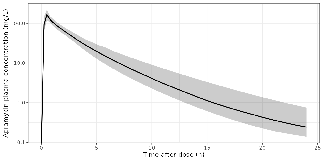

Simulated plasma profiles for 100 subjects at 30 mg/kg (median and 5th-95th percentiles), illustrating the Zhao 2022 IIV block.

Assumptions and deviations

Structural inferences the paper does not print. The source article contains no numbered equations. Figure 1 gives the compartmental schematic and Table 1 gives every parameter with its unit, but the algebraic form of three terms had to be inferred:

• ksr = (kg - kd) * Btot / Bmax. Figure 1 labels ksr as “the transfer from the susceptible to the dormant population as a response to high population densities”, and Table 1 fixes Bmax. This is the standard Nielsen-lineage form and is the only one under which the total count converges to Bmax at stationary phase. The simulated growth controls reach Bmax to within 0.02 log10 in all four in vitro conditions and in both mouse organs, which is the check that would fail if the form were wrong.
• kdrug = Slope * (Cu/MIC)^gamma. The Methods call it “a power model” and Table 1 names the parameters “Rate constant for apramycin effect normalized by MIC” with unit 1/h and a separate gamma “Power on drug effect” fixed to 1.
• kada * (Cu/MIC) for the transfer from subpopulation 1 to subpopulation 2. This one is a reconstruction, not a printed equation, and is flagged as such in the model file at the line that implements it. The Methods describe it as “drug-driven”, and Table 1 gives kada in 1/h, so the multiplier must be dimensionless: the MIC-normalized concentration is the only such quantity in the model. A plain first-order transfer would not be drug-driven – and would let resistance emerge in the untreated growth-control arms, which the data contradict; a transfer proportional to the raw concentration would leave kada in L/(mg h), contradicting the table.

Figure 1 shows no arrow for the kada transfer at all, and its legend does not list kada; the transfer is described only in the Methods text. Because that term is inferred rather than transcribed, it is worth stating plainly which observations test it. Four claims the paper makes, none of which was used to build the reconstruction, are reproduced by it:

1. The in vitro growth controls plateau at the tabulated Bmax of 9.18 log10 CFU/mL (asserted in the in vitro checks chunk above).
2. The sharp one. EN591 at 4 x MIC regrows by 28 h at pH 7.4 (to 5.9 log10) but is held down at pH 6 (0.4 log10) – which is precisely the observation the Results cite as their reason for giving that strain pH-specific drug-effect parameters. This split does not appear if the kada form is wrong.
3. The in vivo kidney growth control plateaus at the tabulated Bmax,k of 6.49 log10 CFU/organ.
4. Doses of at least 10 mg/kg twice daily achieve bacterial stasis, matching the Results statement.

The two antecedent papers that might have printed the term explicitly could not be obtained; see the Errata below.

The kada x 1000 row. Table 1 tabulates the in vitro adaptive-resistance rate constant under the row label kada x 1000, so the packaged values are the printed numbers divided by 1000 (8.0e-5, 2.8e-5 and 2.10e-4 /h). The Results text settles the direction: it states that kada was “notably higher in vivo than in vitro”, and the in vivo estimates are 0.031 and 1.35 /h. Those exceed 8.0e-5 but would be lower than the printed 0.080, so the divide-by-1000 reading is the only self-consistent one.

Residual error on the colony counts is not reported. The Methods state that “for residual unexplained variability, additive error models were used”, but no sigma appears in Table 1, in the text, or in the supplement. Rather than invent a magnitude, addSd, addSd_cfuKidney and addSd_cfuBladder are fixed to 0, so the packaged models simulate the typical bacterial time course without observation noise. A user who wants stochastic colony counts must supply their own value. The plasma residual errors are reported and are carried: 49% proportional for the mouse (Sou 2021) and 8.79% proportional for the human (Zhao 2022).

Inter-individual variability. Neither the in vitro model nor the mouse model carries any: none is reported for the pharmacodynamic parameters, and Sou 2021 Table 1 reports no IIV for the mouse PK. The human model carries the four IIV terms and three correlations of Zhao 2022 Table 2. Zhao 2022 additionally estimated inter-individual variability on the residual error (69.5% CV); that term is not carried here, because it affects only the simulated plasma observation noise and never the concentration that drives the bacterial ODEs. Parameter uncertainty from the sampling-importance resampling, which the paper’s Figures 4 and 5 include as shaded bands, is likewise not carried; the simulations above are typical-value traces, so they track the paper’s medians rather than its confidence bands.

Which Zhao 2022 model. Zhao 2022 reports two parameter sets, one fitted to plasma alone and one to plasma and urine jointly. The packaged model uses the plasma+urine column, which the source paper calls its final model and on which it based its model evaluations. The two sets differ by at most 10% (15% for the IIV on V3), so the choice is immaterial to the plasma profile; using the plasma+urine set additionally makes the renal fractional excretion Fe available, which is why the urine compartment is present.

Renal-function wording. Hernandez-Lozano 2025 describes the simulated human as having a “creatinine clearance of 120 mL/min”. The covariate the Zhao 2022 model actually consumes is absolute (non-BSA-normalized) CKD-EPI eGFR, so 120 is entered as CRCL in absolute mL/min. The CRCL canonical accepts both forms; the covariateData note records which one applies.

Mouse body weight. The PK layer scales allometrically from a 70 kg reference, so a weight is required. The Supplementary methods give a mean of 16.8 g for the C3H/HeJ mice of this study, which is the default. The paper’s separate PBPK cross-check used a 20 g mouse instead; that PBPK model was built in PK-Sim, is not described parametrically in the paper, and is not packaged here.

Model time origin (mouse). The in vivo initial densities Inoc_k and Inoc_b are described in the Results as the burden “at 6 h after inoculation”, which is the first sampling time. Model time zero in the mouse file is therefore 6 h after inoculation, and the vignette adds 6 h when plotting against the paper’s “time after inoculation” axis.

Study 3. The ATCC 700336 validation cohort run at Pharmacology Discovery Services Taiwan was infected 96 h rather than 24 h before treatment and used a 10^9 CFU target inoculum, yet the paper applied the same Inoc and the same drug-effect parameters (“Drug effect parameters in both the kidneys and bladder were shared for both cUTI mouse models without a significant impact on model fit”). This vignette simulates only the primary 24 h-infection design of Figure 3; reproducing Figure 4b requires shifting the dose times, which the packaged model supports through the event table.

Errata and unresolved discrepancies

• The Discussion’s “up to 91%” does not recompute. For EN591 the net-growth reduction from knet = kg - kd is 88.5% in the kidney and 76.0% in the bladder, against the Discussion’s “up to 91% for EN591”. The abstract’s own range of “76%-98%” is reproduced exactly, and the bladder value of 76% matches the Results text to the digit, so the 91% appears to be an isolated rounding or transcription slip in the Discussion rather than a different definition of knet.
• The stasis threshold is more conservative than the model. The paper concludes that a single 10.8 mg/kg dose is “sufficient to result in stasis for both strains”, and that in mice “a dose of at least 10 mg/kg twice daily (i.e. 20 mg/kg daily) was enough to achieve bacterial stasis”. The typical-value traces above already fall below their starting burden at lower doses (all human arms except EN591 kidney at 0.3 mg/kg; all mouse arms). The paper’s Figures 3 and 5 show wide uncertainty bands whose upper edge rises above baseline at the low doses, so the recommendation appears to be based on the full simulated distribution rather than the median. Because the parameter uncertainty is not packaged, this vignette validates the medians against the published median lines instead of re-deriving the threshold.
• Table 1 typography. The 95% confidence interval for the in vitro SlopeS of ATCC 700336 is printed as “2.38.3.80”; it is read here as 2.38 to 3.80. The interval is documentation only and no packaged value depends on it.
• The two antecedents that might print the kada equation could not be obtained. Aranzana-Climent 2022 (reference 26, Clin Microbiol Infect, doi:10.1016/j.cmi.2022.05.003) and Minichmayr 2022 (reference 24, Int J Antimicrob Agents, doi:10.1016/j.ijantimicag.2022.106616 – the paper cited at the kada sentence itself) are both Elsevier titles outside the PMC open-access subset, and every automated route returned an IP block rather than a document. Neither is on disk, so neither was read, and nothing in this vignette rests on their contents. They are logged in the ingestion project’s needs_acquisition.jsonl at corroborative severity: obtaining them would confirm the kada equation form recorded above, not supply any missing number. Every numeric value packaged in the three model files comes from Hernandez-Lozano 2025 itself or from the two upstream PK papers that are on disk (Sou 2021, Zhao 2022). In particular, the two unbound fractions for which Aranzana-Climent 2022 is cited (91.6% mouse, 92.9% human) are quoted directly in the Hernandez-Lozano 2025 Methods text and were taken from there.

Session information

sessionInfo()
#> R version 4.6.1 (2026-06-24)
#> Platform: x86_64-pc-linux-gnu
#> Running under: Ubuntu 24.04.4 LTS
#> 
#> Matrix products: default
#> BLAS:   /usr/lib/x86_64-linux-gnu/openblas-pthread/libblas.so.3 
#> LAPACK: /usr/lib/x86_64-linux-gnu/openblas-pthread/libopenblasp-r0.3.26.so;  LAPACK version 3.12.0
#> 
#> locale:
#>  [1] LC_CTYPE=C.UTF-8       LC_NUMERIC=C           LC_TIME=C.UTF-8       
#>  [4] LC_COLLATE=C.UTF-8     LC_MONETARY=C.UTF-8    LC_MESSAGES=C.UTF-8   
#>  [7] LC_PAPER=C.UTF-8       LC_NAME=C              LC_ADDRESS=C          
#> [10] LC_TELEPHONE=C         LC_MEASUREMENT=C.UTF-8 LC_IDENTIFICATION=C   
#> 
#> time zone: UTC
#> tzcode source: system (glibc)
#> 
#> attached base packages:
#> [1] stats     graphics  grDevices utils     datasets  methods   base     
#> 
#> other attached packages:
#> [1] ggplot2_4.0.3         tidyr_1.3.2           dplyr_1.2.1          
#> [4] rxode2_5.1.6          PKNCA_0.12.1          nlmixr2lib_0.3.2.9000
#> 
#> loaded via a namespace (and not attached):
#>  [1] gtable_0.3.6        xfun_0.60           bslib_0.12.0       
#>  [4] lattice_0.22-9      vctrs_0.7.3         tools_4.6.1        
#>  [7] generics_0.1.4      parallel_4.6.1      tibble_3.3.1       
#> [10] symengine_0.2.13    pkgconfig_2.0.3     data.table_1.18.6.1
#> [13] checkmate_2.3.4     RColorBrewer_1.1-3  S7_0.2.2           
#> [16] desc_1.4.3          RcppParallel_6.2.1  lifecycle_1.0.5    
#> [19] compiler_4.6.1      farver_2.1.2        textshaping_1.0.5  
#> [22] fontawesome_0.5.3   htmltools_0.5.9     sys_3.4.3          
#> [25] sass_0.4.10         yaml_2.3.12         pillar_1.11.1      
#> [28] pkgdown_2.2.1       crayon_1.5.3        jquerylib_0.1.4    
#> [31] whisker_0.4.1       openssl_2.4.2       cachem_1.1.0       
#> [34] nlme_3.1-169        tidyselect_1.2.1    digest_0.6.39      
#> [37] lotri_1.0.4         purrr_1.2.2         labeling_0.4.3     
#> [40] rxode2ll_2.0.16     fastmap_1.2.0       grid_4.6.1         
#> [43] cli_3.6.6           dparser_1.3.1-13    magrittr_2.0.5     
#> [46] withr_3.0.3         scales_1.4.0        backports_1.5.1    
#> [49] rmarkdown_2.31      otel_0.2.0          askpass_1.2.1      
#> [52] ragg_1.5.2          memoise_2.0.1       evaluate_1.0.5     
#> [55] knitr_1.51          rex_1.2.2           PreciseSums_0.7    
#> [58] rlang_1.3.0         downlit_0.4.5       Rcpp_1.1.2         
#> [61] glue_1.8.1          xml2_1.6.0          jsonlite_2.0.0     
#> [64] R6_2.6.1            systemfonts_1.3.2   fs_2.1.0