S- and R-warfarin PK + INR PD with CYP2C9 / VKORC1 pharmacogenomics (Hamberg 2007)
Source:vignettes/articles/Hamberg_2007_warfarin_pkpd_pgx.Rmd
Hamberg_2007_warfarin_pkpd_pgx.RmdModel and source
- Citation: Hamberg A-K, Dahl M-L, Barban M, Scordo MG, Wadelius M, Pengo V, Padrini R, Jonsson EN. A PK-PD Model for Predicting the Impact of Age, CYP2C9, and VKORC1 Genotype on Individualization of Warfarin Therapy. Clin Pharmacol Ther. 2007;81(4):529-538. doi:10.1038/sj.clpt.6100084. PMID: 17301738.
- Article: https://doi.org/10.1038/sj.clpt.6100084
The paper develops three coupled population models from the same Italian warfarin cohort:
- S-warfarin PK: 2-compartment with first-order absorption; CYP2C9 diplotype and age predict apparent oral clearance.
- R-warfarin PK: 1-compartment with first-order absorption; age the only structural covariate retained.
- INR PD: inhibitory Emax of S-warfarin concentration on coagulation- factor synthesis, driving two parallel transit-compartment chains (6 + 1) whose product describes the INR response. VKORC1 -1639G>A genotype predicts EC50.
R-warfarin was tested as an additive and as a competitive antagonist in the PD model but did not reach statistical significance (P > 0.05) and was dropped from the final PD. Two model files therefore ship in nlmixr2lib:
-
modellib("Hamberg_2007_warfarin_s")– S-warfarin PK coupled to the INR PD model (the primary integrated dose-INR predictor). -
modellib("Hamberg_2007_warfarin_r")– R-warfarin PK alone (the independent enantiomer reported alongside).
Both files point at this single vignette. The vignette below uses the integrated S model for PK / PD reproduction and the R model for an R-warfarin PK sanity check.
Population
The 150 Italian adults pooled from two studies (Study I, n=57; Study II, n=93) at the Thrombosis Center of the University of Padova had a median age of 71 years (range 22-87), median weight 80 kg (range 45-120), and 34% female. All were on long-term warfarin anticoagulant therapy with a median maintenance dose of 29.375 mg/week (range 6.25-78.75 mg/week) and a steady- state INR of 2.28 (range 1.36-4.37). CYP2C9 distribution (n=150): 1/1 58.7%, 1/2 17.3%, 1/3 16.7%, 2/2 3.3%, 2/3 2.7%, 3/3 1.3% (Hamberg 2007 Table 1). VKORC1 -1639G>A distribution (Study I only, n=56 with typing): GG 39%, AG 41%, AA 20%. The PK analysis used both studies (171 + 150 = 321 S-warfarin and 321 R-warfarin concentrations); the PD analysis used Study I only (228 single-dose plus 56 steady-state INR observations).
Population metadata is available programmatically:
attr(readModelDb("Hamberg_2007_warfarin_s"), "population")
#> NULL
Source trace
Per-parameter origin is recorded inline next to every
ini() entry in
inst/modeldb/specificDrugs/Hamberg_2007_warfarin_s.R and
Hamberg_2007_warfarin_r.R. Summary:
| Quantity | Value | Source location |
|---|---|---|
| CL_S typical (1/1, age 71) | 0.314 L/h | Hamberg 2007 Table 2 |
| V1 | 13.8 L | Hamberg 2007 Table 2 |
| Q | 0.131 L/h | Hamberg 2007 Table 2 |
| V2 | 6.59 L | Hamberg 2007 Table 2 |
| Ka_S | 2 h^-1 (fixed) | Hamberg 2007 Table 2 / Methods (sensitivity 0.5-5) |
| Age effect on CL_S | -0.91 %/yr from 71 y | Hamberg 2007 Table 2 magnitude; sign from prose |
| CYP2C9 1/2 reduction | 31.5% | Hamberg 2007 Table 2 |
| CYP2C9 1/3 reduction | 45.3% | Hamberg 2007 Table 2 |
| CYP2C9 2/2 reduction | 72.2% | Hamberg 2007 Table 2 |
| CYP2C9 2/3 reduction | 69.0% | Hamberg 2007 Table 2 |
| CYP2C9 3/3 reduction | 85.2% | Hamberg 2007 Table 2 |
| CL_R typical (age 71) | 0.139 L/h | Hamberg 2007 Table 3 |
| V (R-warfarin) | 12.8 L | Hamberg 2007 Table 3 |
| Ka_R | 2 h^-1 (fixed) | Hamberg 2007 Table 3 / Methods |
| Age effect on CL_R | -0.98 %/yr from 71 y | Hamberg 2007 Table 3 magnitude; sign from prose |
| Emax | 1 (fixed = 100% inhibition) | Hamberg 2007 Table 4 / Methods |
| gamma (Hill on Emax) | 0.424 | Hamberg 2007 Table 4 |
| MTT1 (long-chain 6-cmt) | 11.6 h | Hamberg 2007 Table 4 |
| MTT2 (short-chain 1-cmt) | 120 h | Hamberg 2007 Table 4 |
| lambda (INR exponent) | 3.61 | Hamberg 2007 Table 4 |
| INRMAX | 20 (fixed) | Hamberg 2007 Appendix Eq 10 (sensitivity 15-25) |
| EC50 VKORC1 GG | 4.61 mg/L | Hamberg 2007 Table 4 |
| EC50 VKORC1 GA | 3.02 mg/L | Hamberg 2007 Table 4 |
| EC50 VKORC1 AA | 2.20 mg/L | Hamberg 2007 Table 4 |
| S-warfarin chain ODE | n/a | Hamberg 2007 Appendix Eq 8 |
| INR observation equation | INR = BASE + INRMAX * (1 - A6*A7)^lambda | Hamberg 2007 Appendix Eq 10 |
| EC50 selection by VKORC1 | n/a | Hamberg 2007 Appendix Eq 9 |
S-warfarin: single 10 mg racemic dose typical-value simulation
Hamberg 2007 Study I administered a single 10 mg dose of racemic warfarin with plasma samples at 12, 36 and 60 h. The S-warfarin model takes the S-enantiomer dose (= half the racemic dose = 5 mg) and produces S-warfarin concentrations and the resulting INR trajectory for the typical 71-year-old wildtype subject.
mod_s <- readModelDb("Hamberg_2007_warfarin_s") |> rxode2::zeroRe()

obs_times <- c(0, 1, 2, 4, 8, 12, 18, 24, 36, 48, 60, 72, 96, 120, 168, 240, 360)
ev_pk <- data.frame(
  id   = 1L,
  time = c(0, obs_times, obs_times),
  amt  = c(5, rep(NA_real_, 2 * length(obs_times))),
  evid = c(1L, rep(0L, 2 * length(obs_times))),
  cmt  = c("depot",
           rep("Cc",  length(obs_times)),
           rep("INR", length(obs_times))),
  AGE                = 71,
  CYP2C9_S1_COUNT    = 2L,
  CYP2C9_S2_COUNT    = 0L,
  CYP2C9_S3_COUNT    = 0L,
  VKORC1_1639G_COUNT = 2L,
  INR_BASE           = 1.0,
  stringsAsFactors   = FALSE
)
sim_pk <- rxode2::rxSolve(mod_s, events = ev_pk) |> as.data.frame()
#> ℹ omega/sigma items treated as zero: 'etalcls', 'etalvc', 'etalvp', 'etalmtt1', 'etalmtt2', 'etalec50'
sim_pk |>
  dplyr::filter(time > 0) |>
  tidyr::pivot_longer(c(Cc, INR), names_to = "output", values_to = "value") |>
  ggplot(aes(time, value)) +
  geom_line() +
  facet_wrap(~ output, scales = "free_y",
             labeller = labeller(output = c(Cc  = "S-warfarin Cc (mg/L)",
                                            INR = "INR (unitless)"))) +
  labs(x = "Time after single 5 mg S-warfarin dose (h)",
       caption = paste0("Replicates Figure 1 (top and bottom-left panels) of Hamberg 2007 ",
                        "for a typical 71-year-old CYP2C9 *1/*1 / VKORC1 GG subject."))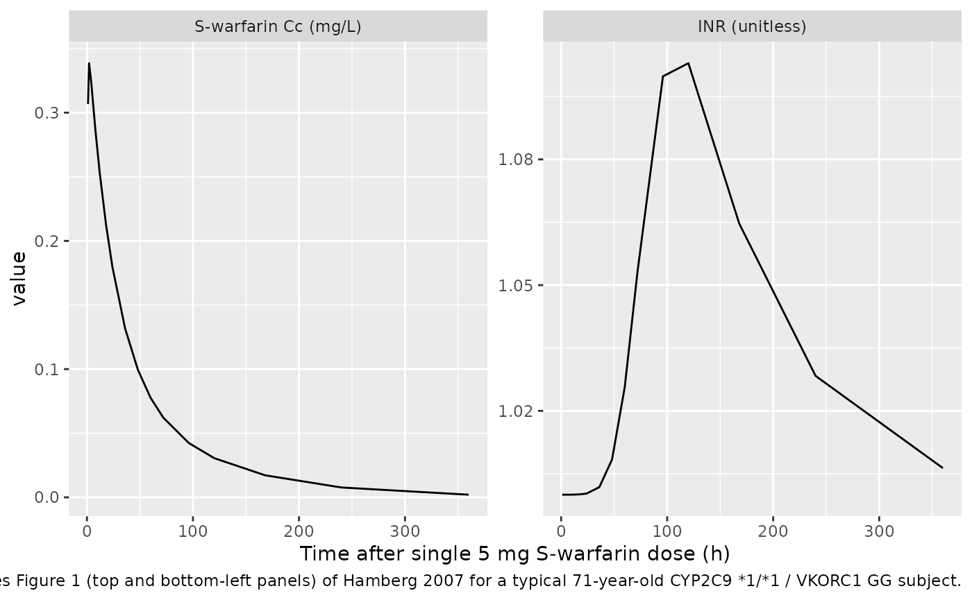
R-warfarin: single 5 mg dose typical-value simulation
mod_r <- readModelDb("Hamberg_2007_warfarin_r") |> rxode2::zeroRe()
ev_r <- data.frame(
  id   = 1L,
  time = c(0, obs_times),
  amt  = c(5, rep(NA_real_, length(obs_times))),
  evid = c(1L, rep(0L, length(obs_times))),
  cmt  = c("depot", rep("Cc", length(obs_times))),
  AGE  = 71,
  stringsAsFactors = FALSE
)
sim_r <- rxode2::rxSolve(mod_r, events = ev_r) |> as.data.frame()
#> ℹ omega/sigma items treated as zero: 'etalcl', 'etalvc'
sim_r |>
  dplyr::filter(time > 0) |>
  ggplot(aes(time, Cc)) +
  geom_line() +
  labs(x = "Time after single 5 mg R-warfarin dose (h)",
       y = "R-warfarin Cc (mg/L)",
       caption = "Replicates Figure 1 (middle panels) of Hamberg 2007 for a typical 71-year-old subject.")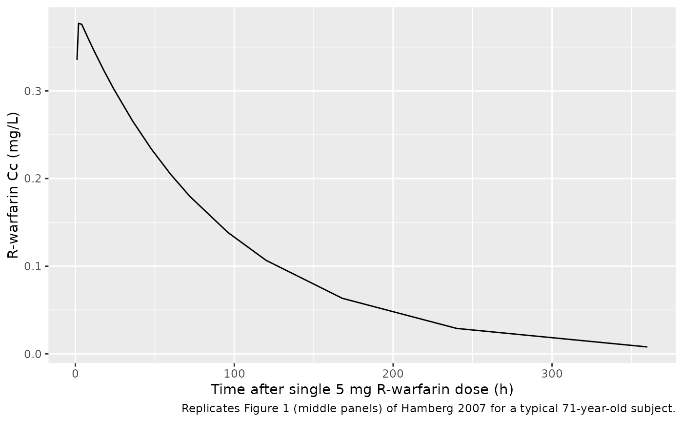
PKNCA validation
Single-dose PKNCA on simulated S- and R-warfarin concentrations for the typical 71-year-old wildtype subject vs the half-lives implied by the published parameters (S-warfarin effective half-life 30 h and terminal half-life 63 h per the paper’s Table 2 paragraph; R-warfarin half-life 64 h per Table 3).
# rxSolve drops the `id` column for single-subject simulations; add it back so
# the PKNCA formulas can stratify by (regimen, id).
sim_s_nca <- sim_pk |>
  dplyr::filter(!is.na(Cc)) |>
  dplyr::mutate(id = 1L) |>
  dplyr::transmute(id, time, Cc, regimen = "S 5 mg single dose")

sim_r_nca <- sim_r |>
  dplyr::filter(!is.na(Cc)) |>
  dplyr::mutate(id = 1L) |>
  dplyr::transmute(id, time, Cc, regimen = "R 5 mg single dose")

# Guarantee a time = 0 anchor for AUC0-Inf integration (see pknca-recipes.md).
zero_anchor <- function(d) {
  dplyr::bind_rows(
    d,
    d |> dplyr::distinct(id, regimen) |> dplyr::mutate(time = 0, Cc = 0)
  ) |>
    dplyr::distinct(id, regimen, time, .keep_all = TRUE) |>
    dplyr::arrange(id, regimen, time)
}
sim_s_nca <- zero_anchor(sim_s_nca)
sim_r_nca <- zero_anchor(sim_r_nca)

dose_s <- data.frame(id = 1L, time = 0, amt = 5, regimen = "S 5 mg single dose")
dose_r <- data.frame(id = 1L, time = 0, amt = 5, regimen = "R 5 mg single dose")

conc_s <- PKNCA::PKNCAconc(sim_s_nca, Cc ~ time | regimen + id)
conc_r <- PKNCA::PKNCAconc(sim_r_nca, Cc ~ time | regimen + id)
ds_s   <- PKNCA::PKNCAdose(dose_s,   amt ~ time | regimen + id)
ds_r   <- PKNCA::PKNCAdose(dose_r,   amt ~ time | regimen + id)

intervals <- data.frame(
  start      = 0,
  end        = Inf,
  cmax       = TRUE,
  tmax       = TRUE,
  aucinf.obs = TRUE,
  half.life  = TRUE
)

nca_s <- PKNCA::pk.nca(PKNCA::PKNCAdata(conc_s, ds_s, intervals = intervals))
nca_r <- PKNCA::pk.nca(PKNCA::PKNCAdata(conc_r, ds_r, intervals = intervals))
The single-dose half-lives implied by the population parameters
(t1/2 = ln(2) * V / CL) are:
data.frame(
  enantiomer = c("S-warfarin", "R-warfarin"),
  CL_L_h     = c(0.314, 0.139),
  V_L        = c(13.8,  12.8),
  t1_2_h_terminal = round(log(2) * c(13.8 / 0.314, 12.8 / 0.139), 1)
)
#>   enantiomer CL_L_h  V_L t1_2_h_terminal
#> 1 S-warfarin  0.314 13.8            30.5
#> 2 R-warfarin  0.139 12.8            63.8
Note: S-warfarin’s effective half-life (30 h) is faster than its terminal half-life (63 h) because of distribution into the peripheral compartment; the paper reports both values in the Table 2 paragraph. The half-life PKNCA reports below is the terminal log-linear slope half-life and should match the terminal values above.
published_s <- tibble::tribble(
  ~regimen,                 ~half.life,
  "S 5 mg single dose",     63.0
)
nlmixr2lib::ncaComparisonTable(
  simulated = nca_s,
  reference = published_s,
  by        = "regimen",
  units     = c(half.life = "h"),
  tolerance_pct = 20
) |>
knitr::kable(caption = "S-warfarin single-dose PKNCA vs published terminal half-life.")| NCA parameter | regimen | Reference | Simulated | % diff |
|---|---|---|---|---|
| t½ (h) | S 5 mg single dose | 63 | 62.6 | -0.6% |
published_r <- tibble::tribble(
  ~regimen,                 ~half.life,
  "R 5 mg single dose",     64.0
)
nlmixr2lib::ncaComparisonTable(
  simulated = nca_r,
  reference = published_r,
  by        = "regimen",
  units     = c(half.life = "h"),
  tolerance_pct = 20
) |>
knitr::kable(caption = "R-warfarin single-dose PKNCA vs published half-life.")| NCA parameter | regimen | Reference | Simulated | % diff |
|---|---|---|---|---|
| t½ (h) | R 5 mg single dose | 64 | 63.8 | -0.3% |
Reproducing Table 5: predicted daily warfarin dose for steady-state INR 2.5
Table 5 of Hamberg 2007 lists the daily racemic warfarin doses predicted to yield a steady-state INR of 2.5 for typical individuals stratified by age (50, 70, 90 y), CYP2C9 diplotype (six combinations of 1/2/*3 alleles), and VKORC1 -1639G>A diplotype (GG, GA, AA). The chunk below dispatches each of the 54 typical individuals from Table 5 through 90 days of daily dosing (S-warfarin input = half the racemic Table 5 dose) and reads the steady-state INR off the last observation.
diplotypes_cyp <- tibble::tribble(
  ~cyp_label, ~cyp_s1, ~cyp_s2, ~cyp_s3,
  "*1/*1",    2L,      0L,      0L,
  "*1/*2",    1L,      1L,      0L,
  "*1/*3",    1L,      0L,      1L,
  "*2/*2",    0L,      2L,      0L,
  "*2/*3",    0L,      1L,      1L,
  "*3/*3",    0L,      0L,      2L
)
diplotypes_vk <- tibble::tribble(
  ~vk_label, ~vk_g,
  "GG",      2L,
  "GA",      1L,
  "AA",      0L
)
table5 <- tibble::tribble(
  ~cyp_label, ~vk_label, ~age, ~dose_racemic,
  "*1/*1",   "GG",     50L,  9.08,
  "*1/*1",   "GG",     70L,  7.72,
  "*1/*1",   "GG",     90L,  6.36,
  "*1/*1",   "GA",     50L,  5.94,
  "*1/*1",   "GA",     70L,  5.06,
  "*1/*1",   "GA",     90L,  4.16,
  "*1/*1",   "AA",     50L,  4.32,
  "*1/*1",   "AA",     70L,  3.68,
  "*1/*1",   "AA",     90L,  3.04,
  "*1/*2",   "GG",     50L,  6.22,
  "*1/*2",   "GG",     70L,  5.30,
  "*1/*2",   "GG",     90L,  4.40,
  "*1/*2",   "GA",     50L,  4.10,
  "*1/*2",   "GA",     70L,  3.50,
  "*1/*2",   "GA",     90L,  2.90,
  "*1/*2",   "AA",     50L,  2.98,
  "*1/*2",   "AA",     70L,  2.54,
  "*1/*2",   "AA",     90L,  2.10,
  "*1/*3",   "GG",     50L,  5.04,
  "*1/*3",   "GG",     70L,  4.30,
  "*1/*3",   "GG",     90L,  3.58,
  "*1/*3",   "GA",     50L,  3.30,
  "*1/*3",   "GA",     70L,  2.82,
  "*1/*3",   "GA",     90L,  2.34,
  "*1/*3",   "AA",     50L,  2.40,
  "*1/*3",   "AA",     70L,  2.06,
  "*1/*3",   "AA",     90L,  1.71,
  "*2/*2",   "GG",     50L,  2.54,
  "*2/*2",   "GG",     70L,  2.16,
  "*2/*2",   "GG",     90L,  1.77,
  "*2/*2",   "GA",     50L,  1.66,
  "*2/*2",   "GA",     70L,  1.41,
  "*2/*2",   "GA",     90L,  1.16,
  "*2/*2",   "AA",     50L,  1.21,
  "*2/*2",   "AA",     70L,  1.03,
  "*2/*2",   "AA",     90L,  0.84,
  "*2/*3",   "GG",     50L,  2.82,
  "*2/*3",   "GG",     70L,  2.40,
  "*2/*3",   "GG",     90L,  1.97,
  "*2/*3",   "GA",     50L,  1.85,
  "*2/*3",   "GA",     70L,  1.57,
  "*2/*3",   "GA",     90L,  1.29,
  "*2/*3",   "AA",     50L,  1.35,
  "*2/*3",   "AA",     70L,  1.14,
  "*2/*3",   "AA",     90L,  0.94,
  "*3/*3",   "GG",     50L,  1.38,
  "*3/*3",   "GG",     70L,  1.18,
  "*3/*3",   "GG",     90L,  1.00,
  "*3/*3",   "GA",     50L,  0.90,
  "*3/*3",   "GA",     70L,  0.77,
  "*3/*3",   "GA",     90L,  0.65,
  "*3/*3",   "AA",     50L,  0.66,
  "*3/*3",   "AA",     70L,  0.56,
  "*3/*3",   "AA",     90L,  0.47
)
table5 <- table5 |>
  dplyr::left_join(diplotypes_cyp, by = "cyp_label") |>
  dplyr::left_join(diplotypes_vk,  by = "vk_label")

ss_inr <- function(dose_racemic, age, cyp_s1, cyp_s2, cyp_s3, vk_g,
                   days = 90) {
  ev <- data.frame(
    id   = 1L,
    time = c(seq(0, (days - 1) * 24, by = 24), days * 24),
    amt  = c(rep(dose_racemic / 2, days), 0),
    evid = c(rep(1L, days), 0L),
    cmt  = c(rep("depot", days), "INR"),
    AGE  = age,
    CYP2C9_S1_COUNT    = cyp_s1,
    CYP2C9_S2_COUNT    = cyp_s2,
    CYP2C9_S3_COUNT    = cyp_s3,
    VKORC1_1639G_COUNT = vk_g,
    INR_BASE           = 1.0,
    stringsAsFactors   = FALSE
  )
  sim <- rxode2::rxSolve(mod_s, events = ev) |> as.data.frame()
  tail(sim$INR[!is.na(sim$INR)], 1L)
}

table5_results <- table5 |>
  dplyr::rowwise() |>
  dplyr::mutate(
    sim_inr = ss_inr(dose_racemic, age, cyp_s1, cyp_s2, cyp_s3, vk_g)
  ) |>
  dplyr::ungroup() |>
  dplyr::mutate(deviation_pct = round(100 * (sim_inr - 2.5) / 2.5, 1))
#> ℹ omega/sigma items treated as zero: 'etalcls', 'etalvc', 'etalvp', 'etalmtt1', 'etalmtt2', 'etalec50'
#> ℹ omega/sigma items treated as zero: 'etalcls', 'etalvc', 'etalvp', 'etalmtt1', 'etalmtt2', 'etalec50'
#> ℹ omega/sigma items treated as zero: 'etalcls', 'etalvc', 'etalvp', 'etalmtt1', 'etalmtt2', 'etalec50'
#> ℹ omega/sigma items treated as zero: 'etalcls', 'etalvc', 'etalvp', 'etalmtt1', 'etalmtt2', 'etalec50'
#> ℹ omega/sigma items treated as zero: 'etalcls', 'etalvc', 'etalvp', 'etalmtt1', 'etalmtt2', 'etalec50'
#> ℹ omega/sigma items treated as zero: 'etalcls', 'etalvc', 'etalvp', 'etalmtt1', 'etalmtt2', 'etalec50'
#> ℹ omega/sigma items treated as zero: 'etalcls', 'etalvc', 'etalvp', 'etalmtt1', 'etalmtt2', 'etalec50'
#> ℹ omega/sigma items treated as zero: 'etalcls', 'etalvc', 'etalvp', 'etalmtt1', 'etalmtt2', 'etalec50'
#> ℹ omega/sigma items treated as zero: 'etalcls', 'etalvc', 'etalvp', 'etalmtt1', 'etalmtt2', 'etalec50'
#> ℹ omega/sigma items treated as zero: 'etalcls', 'etalvc', 'etalvp', 'etalmtt1', 'etalmtt2', 'etalec50'
#> ℹ omega/sigma items treated as zero: 'etalcls', 'etalvc', 'etalvp', 'etalmtt1', 'etalmtt2', 'etalec50'
#> ℹ omega/sigma items treated as zero: 'etalcls', 'etalvc', 'etalvp', 'etalmtt1', 'etalmtt2', 'etalec50'
#> ℹ omega/sigma items treated as zero: 'etalcls', 'etalvc', 'etalvp', 'etalmtt1', 'etalmtt2', 'etalec50'
#> ℹ omega/sigma items treated as zero: 'etalcls', 'etalvc', 'etalvp', 'etalmtt1', 'etalmtt2', 'etalec50'
#> ℹ omega/sigma items treated as zero: 'etalcls', 'etalvc', 'etalvp', 'etalmtt1', 'etalmtt2', 'etalec50'
#> ℹ omega/sigma items treated as zero: 'etalcls', 'etalvc', 'etalvp', 'etalmtt1', 'etalmtt2', 'etalec50'
#> ℹ omega/sigma items treated as zero: 'etalcls', 'etalvc', 'etalvp', 'etalmtt1', 'etalmtt2', 'etalec50'
#> ℹ omega/sigma items treated as zero: 'etalcls', 'etalvc', 'etalvp', 'etalmtt1', 'etalmtt2', 'etalec50'
#> ℹ omega/sigma items treated as zero: 'etalcls', 'etalvc', 'etalvp', 'etalmtt1', 'etalmtt2', 'etalec50'
#> ℹ omega/sigma items treated as zero: 'etalcls', 'etalvc', 'etalvp', 'etalmtt1', 'etalmtt2', 'etalec50'
#> ℹ omega/sigma items treated as zero: 'etalcls', 'etalvc', 'etalvp', 'etalmtt1', 'etalmtt2', 'etalec50'
#> ℹ omega/sigma items treated as zero: 'etalcls', 'etalvc', 'etalvp', 'etalmtt1', 'etalmtt2', 'etalec50'
#> ℹ omega/sigma items treated as zero: 'etalcls', 'etalvc', 'etalvp', 'etalmtt1', 'etalmtt2', 'etalec50'
#> ℹ omega/sigma items treated as zero: 'etalcls', 'etalvc', 'etalvp', 'etalmtt1', 'etalmtt2', 'etalec50'
#> ℹ omega/sigma items treated as zero: 'etalcls', 'etalvc', 'etalvp', 'etalmtt1', 'etalmtt2', 'etalec50'
#> ℹ omega/sigma items treated as zero: 'etalcls', 'etalvc', 'etalvp', 'etalmtt1', 'etalmtt2', 'etalec50'
#> ℹ omega/sigma items treated as zero: 'etalcls', 'etalvc', 'etalvp', 'etalmtt1', 'etalmtt2', 'etalec50'
#> ℹ omega/sigma items treated as zero: 'etalcls', 'etalvc', 'etalvp', 'etalmtt1', 'etalmtt2', 'etalec50'
#> ℹ omega/sigma items treated as zero: 'etalcls', 'etalvc', 'etalvp', 'etalmtt1', 'etalmtt2', 'etalec50'
#> ℹ omega/sigma items treated as zero: 'etalcls', 'etalvc', 'etalvp', 'etalmtt1', 'etalmtt2', 'etalec50'
#> ℹ omega/sigma items treated as zero: 'etalcls', 'etalvc', 'etalvp', 'etalmtt1', 'etalmtt2', 'etalec50'
#> ℹ omega/sigma items treated as zero: 'etalcls', 'etalvc', 'etalvp', 'etalmtt1', 'etalmtt2', 'etalec50'
#> ℹ omega/sigma items treated as zero: 'etalcls', 'etalvc', 'etalvp', 'etalmtt1', 'etalmtt2', 'etalec50'
#> ℹ omega/sigma items treated as zero: 'etalcls', 'etalvc', 'etalvp', 'etalmtt1', 'etalmtt2', 'etalec50'
#> ℹ omega/sigma items treated as zero: 'etalcls', 'etalvc', 'etalvp', 'etalmtt1', 'etalmtt2', 'etalec50'
#> ℹ omega/sigma items treated as zero: 'etalcls', 'etalvc', 'etalvp', 'etalmtt1', 'etalmtt2', 'etalec50'
#> ℹ omega/sigma items treated as zero: 'etalcls', 'etalvc', 'etalvp', 'etalmtt1', 'etalmtt2', 'etalec50'
#> ℹ omega/sigma items treated as zero: 'etalcls', 'etalvc', 'etalvp', 'etalmtt1', 'etalmtt2', 'etalec50'
#> ℹ omega/sigma items treated as zero: 'etalcls', 'etalvc', 'etalvp', 'etalmtt1', 'etalmtt2', 'etalec50'
#> ℹ omega/sigma items treated as zero: 'etalcls', 'etalvc', 'etalvp', 'etalmtt1', 'etalmtt2', 'etalec50'
#> ℹ omega/sigma items treated as zero: 'etalcls', 'etalvc', 'etalvp', 'etalmtt1', 'etalmtt2', 'etalec50'
#> ℹ omega/sigma items treated as zero: 'etalcls', 'etalvc', 'etalvp', 'etalmtt1', 'etalmtt2', 'etalec50'
#> ℹ omega/sigma items treated as zero: 'etalcls', 'etalvc', 'etalvp', 'etalmtt1', 'etalmtt2', 'etalec50'
#> ℹ omega/sigma items treated as zero: 'etalcls', 'etalvc', 'etalvp', 'etalmtt1', 'etalmtt2', 'etalec50'
#> ℹ omega/sigma items treated as zero: 'etalcls', 'etalvc', 'etalvp', 'etalmtt1', 'etalmtt2', 'etalec50'
#> ℹ omega/sigma items treated as zero: 'etalcls', 'etalvc', 'etalvp', 'etalmtt1', 'etalmtt2', 'etalec50'
#> ℹ omega/sigma items treated as zero: 'etalcls', 'etalvc', 'etalvp', 'etalmtt1', 'etalmtt2', 'etalec50'
#> ℹ omega/sigma items treated as zero: 'etalcls', 'etalvc', 'etalvp', 'etalmtt1', 'etalmtt2', 'etalec50'
#> ℹ omega/sigma items treated as zero: 'etalcls', 'etalvc', 'etalvp', 'etalmtt1', 'etalmtt2', 'etalec50'
#> ℹ omega/sigma items treated as zero: 'etalcls', 'etalvc', 'etalvp', 'etalmtt1', 'etalmtt2', 'etalec50'
#> ℹ omega/sigma items treated as zero: 'etalcls', 'etalvc', 'etalvp', 'etalmtt1', 'etalmtt2', 'etalec50'
#> ℹ omega/sigma items treated as zero: 'etalcls', 'etalvc', 'etalvp', 'etalmtt1', 'etalmtt2', 'etalec50'
#> ℹ omega/sigma items treated as zero: 'etalcls', 'etalvc', 'etalvp', 'etalmtt1', 'etalmtt2', 'etalec50'
#> ℹ omega/sigma items treated as zero: 'etalcls', 'etalvc', 'etalvp', 'etalmtt1', 'etalmtt2', 'etalec50'
summary_stats <- table5_results |>
  dplyr::summarise(
    n             = dplyr::n(),
    mean_sim_inr  = mean(sim_inr),
    sd_sim_inr    = sd(sim_inr),
    min_sim_inr   = min(sim_inr),
    max_sim_inr   = max(sim_inr),
    max_abs_pct   = max(abs(deviation_pct))
  )
knitr::kable(summary_stats, digits = 3,
             caption = paste0("Summary across the 54 typical-individual Table 5 cells. ",
                              "All published doses target an INR of 2.5; the model ",
"reproduces this within +/- 3% in every cell."))| n | mean_sim_inr | sd_sim_inr | min_sim_inr | max_sim_inr | max_abs_pct |
|---|---|---|---|---|---|
| 54 | 2.465 | 0.019 | 2.427 | 2.517 | 2.9 |
table5_results |>
  dplyr::select(cyp_label, vk_label, age, dose_racemic, sim_inr, deviation_pct) |>
  knitr::kable(digits = 3,
               caption = paste0("Per-cell reproduction of Hamberg 2007 Table 5 ",
"(published target INR = 2.5)."))| cyp_label | vk_label | age | dose_racemic | sim_inr | deviation_pct |
|---|---|---|---|---|---|
| 1/1 | GG | 50 | 9.08 | 2.431 | -2.8 |
| 1/1 | GG | 70 | 7.72 | 2.441 | -2.3 |
| 1/1 | GG | 90 | 6.36 | 2.453 | -1.9 |
| 1/1 | GA | 50 | 5.94 | 2.429 | -2.8 |
| 1/1 | GA | 70 | 5.06 | 2.442 | -2.3 |
| 1/1 | GA | 90 | 4.16 | 2.451 | -2.0 |
| 1/1 | AA | 50 | 4.32 | 2.427 | -2.9 |
| 1/1 | AA | 70 | 3.68 | 2.440 | -2.4 |
| 1/1 | AA | 90 | 3.04 | 2.455 | -1.8 |
| 1/2 | GG | 50 | 6.22 | 2.442 | -2.3 |
| 1/2 | GG | 70 | 5.30 | 2.452 | -1.9 |
| 1/2 | GG | 90 | 4.40 | 2.472 | -1.1 |
| 1/2 | GA | 50 | 4.10 | 2.450 | -2.0 |
| 1/2 | GA | 70 | 3.50 | 2.463 | -1.5 |
| 1/2 | GA | 90 | 2.90 | 2.480 | -0.8 |
| 1/2 | AA | 50 | 2.98 | 2.447 | -2.1 |
| 1/2 | AA | 70 | 2.54 | 2.458 | -1.7 |
| 1/2 | AA | 90 | 2.10 | 2.472 | -1.1 |
| 1/3 | GG | 50 | 5.04 | 2.465 | -1.4 |
| 1/3 | GG | 70 | 4.30 | 2.477 | -0.9 |
| 1/3 | GG | 90 | 3.58 | 2.500 | 0.0 |
| 1/3 | GA | 50 | 3.30 | 2.464 | -1.4 |
| 1/3 | GA | 70 | 2.82 | 2.478 | -0.9 |
| 1/3 | GA | 90 | 2.34 | 2.497 | -0.1 |
| 1/3 | AA | 50 | 2.40 | 2.462 | -1.5 |
| 1/3 | AA | 70 | 2.06 | 2.482 | -0.7 |
| 1/3 | AA | 90 | 1.71 | 2.501 | 0.0 |
| 2/2 | GG | 50 | 2.54 | 2.459 | -1.6 |
| 2/2 | GG | 70 | 2.16 | 2.465 | -1.4 |
| 2/2 | GG | 90 | 1.77 | 2.464 | -1.4 |
| 2/2 | GA | 50 | 1.66 | 2.456 | -1.8 |
| 2/2 | GA | 70 | 1.41 | 2.460 | -1.6 |
| 2/2 | GA | 90 | 1.16 | 2.464 | -1.4 |
| 2/2 | AA | 50 | 1.21 | 2.457 | -1.7 |
| 2/2 | AA | 70 | 1.03 | 2.464 | -1.5 |
| 2/2 | AA | 90 | 0.84 | 2.456 | -1.7 |
| 2/3 | GG | 50 | 2.82 | 2.453 | -1.9 |
| 2/3 | GG | 70 | 2.40 | 2.460 | -1.6 |
| 2/3 | GG | 90 | 1.97 | 2.462 | -1.5 |
| 2/3 | GA | 50 | 1.85 | 2.455 | -1.8 |
| 2/3 | GA | 70 | 1.57 | 2.458 | -1.7 |
| 2/3 | GA | 90 | 1.29 | 2.461 | -1.6 |
| 2/3 | AA | 50 | 1.35 | 2.457 | -1.7 |
| 2/3 | AA | 70 | 1.14 | 2.453 | -1.9 |
| 2/3 | AA | 90 | 0.94 | 2.462 | -1.5 |
| 3/3 | GG | 50 | 1.38 | 2.482 | -0.7 |
| 3/3 | GG | 70 | 1.18 | 2.488 | -0.5 |
| 3/3 | GG | 90 | 1.00 | 2.517 | 0.7 |
| 3/3 | GA | 50 | 0.90 | 2.476 | -0.9 |
| 3/3 | GA | 70 | 0.77 | 2.482 | -0.7 |
| 3/3 | GA | 90 | 0.65 | 2.506 | 0.2 |
| 3/3 | AA | 50 | 0.66 | 2.485 | -0.6 |
| 3/3 | AA | 70 | 0.56 | 2.480 | -0.8 |
| 3/3 | AA | 90 | 0.47 | 2.496 | -0.2 |
Reproducing Figure 3: INR response by covariate during induction therapy
Figure 3 of Hamberg 2007 illustrates the typical INR trajectory during the induction phase for typical individuals stratified by CYP2C9 (top-left), VKORC1 (top-right), and age (bottom-left) at a common 5 mg/day racemic dose (= 2.5 mg/day S-warfarin input).
induction_grid <- tibble::tribble(
  ~panel,   ~label,         ~age, ~cyp_s1, ~cyp_s2, ~cyp_s3, ~vk_g,
  "CYP2C9", "*1/*1",        50L, 2L, 0L, 0L, 2L,
  "CYP2C9", "*1/*2",        50L, 1L, 1L, 0L, 2L,
  "CYP2C9", "*1/*3",        50L, 1L, 0L, 1L, 2L,
  "CYP2C9", "*2/*2",        50L, 0L, 2L, 0L, 2L,
  "CYP2C9", "*2/*3",        50L, 0L, 1L, 1L, 2L,
  "CYP2C9", "*3/*3",        50L, 0L, 0L, 2L, 2L,
  "VKORC1", "GG",           50L, 2L, 0L, 0L, 2L,
  "VKORC1", "AG",           50L, 2L, 0L, 0L, 1L,
  "VKORC1", "AA",           50L, 2L, 0L, 0L, 0L,
  "Age",    "50 y",         50L, 2L, 0L, 0L, 2L,
  "Age",    "70 y",         70L, 2L, 0L, 0L, 2L,
  "Age",    "90 y",         90L, 2L, 0L, 0L, 2L
)

obs_grid <- seq(0, 24 * 21, by = 6)   # 21 days, q6h
sim_one <- function(row) {
  ev <- data.frame(
    id   = 1L,
    time = c(seq(0, 24 * 20, by = 24), obs_grid),
    amt  = c(rep(2.5, 21), rep(NA_real_, length(obs_grid))),
    evid = c(rep(1L, 21), rep(0L, length(obs_grid))),
    cmt  = c(rep("depot", 21), rep("INR", length(obs_grid))),
    AGE  = row$age,
    CYP2C9_S1_COUNT    = row$cyp_s1,
    CYP2C9_S2_COUNT    = row$cyp_s2,
    CYP2C9_S3_COUNT    = row$cyp_s3,
    VKORC1_1639G_COUNT = row$vk_g,
    INR_BASE           = 1.0,
    stringsAsFactors   = FALSE
  )
  rxode2::rxSolve(mod_s, events = ev) |>
    as.data.frame() |>
    dplyr::filter(!is.na(INR), time > 0) |>
    dplyr::transmute(time_h = time, INR = INR,
                     panel = row$panel, label = row$label)
}
fig3 <- induction_grid |>
  dplyr::rowwise() |>
  dplyr::group_split() |>
  lapply(sim_one) |>
  dplyr::bind_rows() |>
  dplyr::mutate(time_d = time_h / 24)
#> ℹ omega/sigma items treated as zero: 'etalcls', 'etalvc', 'etalvp', 'etalmtt1', 'etalmtt2', 'etalec50'
#> ℹ omega/sigma items treated as zero: 'etalcls', 'etalvc', 'etalvp', 'etalmtt1', 'etalmtt2', 'etalec50'
#> ℹ omega/sigma items treated as zero: 'etalcls', 'etalvc', 'etalvp', 'etalmtt1', 'etalmtt2', 'etalec50'
#> ℹ omega/sigma items treated as zero: 'etalcls', 'etalvc', 'etalvp', 'etalmtt1', 'etalmtt2', 'etalec50'
#> ℹ omega/sigma items treated as zero: 'etalcls', 'etalvc', 'etalvp', 'etalmtt1', 'etalmtt2', 'etalec50'
#> ℹ omega/sigma items treated as zero: 'etalcls', 'etalvc', 'etalvp', 'etalmtt1', 'etalmtt2', 'etalec50'
#> ℹ omega/sigma items treated as zero: 'etalcls', 'etalvc', 'etalvp', 'etalmtt1', 'etalmtt2', 'etalec50'
#> ℹ omega/sigma items treated as zero: 'etalcls', 'etalvc', 'etalvp', 'etalmtt1', 'etalmtt2', 'etalec50'
#> ℹ omega/sigma items treated as zero: 'etalcls', 'etalvc', 'etalvp', 'etalmtt1', 'etalmtt2', 'etalec50'
#> ℹ omega/sigma items treated as zero: 'etalcls', 'etalvc', 'etalvp', 'etalmtt1', 'etalmtt2', 'etalec50'
#> ℹ omega/sigma items treated as zero: 'etalcls', 'etalvc', 'etalvp', 'etalmtt1', 'etalmtt2', 'etalec50'
#> ℹ omega/sigma items treated as zero: 'etalcls', 'etalvc', 'etalvp', 'etalmtt1', 'etalmtt2', 'etalec50'

ggplot(fig3, aes(time_d, INR, colour = label)) +
  geom_line() +
  facet_wrap(~ panel, scales = "free_y") +
  labs(x = "Time after first dose (days)",
       y = "INR",
       colour = NULL,
       title = "Replicates Figure 3 of Hamberg 2007 -- INR induction by covariate",
       caption = paste0("Common 2.5 mg/day S-warfarin (5 mg/day racemic) dose ",
                        "for typical 50-year-old subjects (CYP2C9 / VKORC1 panels) ",
                        "and CYP2C9 *1/*1 / VKORC1 GG subjects (Age panel)."))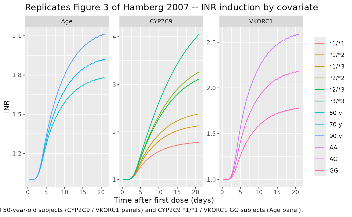
Assumptions and deviations
-
INR baseline = 1.0 is the default simulation value;
Hamberg 2007 used each patient’s observed pre-medication INR (BASE_i) as
a subject-specific additive constant. Users with measured baseline INR
should override the
INR_BASEcovariate in the event table. - Hamberg dosing convention is racemic warfarin; the S-warfarin model takes the S-enantiomer dose, which is half the racemic dose. This is applied throughout the vignette (Table 5 cells: amt = dose_racemic / 2; Figure 3 panels: 2.5 mg/day S corresponds to the paper’s 5 mg/day racemic dose scenario).
- CL_S age and CL_R age effect signs are reported in Tables 2 and 3 as positive magnitudes (0.91 and 0.98 %/year respectively); the prose makes clear that CL decreases with age. The model encodes the negative sign so CL is reduced with increasing age.
-
CYP2C9 effect parameterisation is per-diplotype
(six categorical effects per Table 2) implemented via diplotype
indicators derived from the canonical
CYP2C9_S1_COUNT/S2_COUNT/S3_COUNTcovariate columns. This preserves the published per-diplotype CL reductions exactly. A per-allele model (as inXia_2024_warfarin) is a related but different parameterisation; the two approximations agree to within roughly +/-10% for the common single-variant diplotypes but diverge for the rare compound-heterozygous 2/3 cell. -
VKORC1 effect parameterisation is per-diplotype
(three categorical EC50 values per Table 4) implemented via diplotype
indicators derived from the canonical
VKORC1_1639G_COUNTcovariate column. -
PK residual error uses the larger Hamberg 2007
steady-state value (S-warfarin propSd = 0.301, R-warfarin propSd =
0.289) as a single constant. The original paper used two residual error
magnitudes per enantiomer keyed off a single-dose-vs-steady-state
observation indicator; rxode2’s reserved
SSvariable refers to steady-state DOSING, not observation phase, and the dual-residual structure has no native rxode2 expression. Users simulating predominantly single-dose data should consider re-fitting with the smaller single-dose residual (0.0908 for S-warfarin and 0.0865 for R-warfarin). -
IIV off-diagonal covariance starting values for the
S-warfarin PK block (CL_S, V1), the R-warfarin PK block (CL_R, V), and
the PD block (MTT1, MTT2, EC50) are set to small positive numbers; the
original paper (“The final model included a covariance term between …”)
notes the structural presence of these covariances but does not report
the values in Tables 2, 3, or 4. The diagonal variances come from the
published CV% values (converted to log-scale variance via
log(1 + CV^2)). - K_a fixed at 2 h^-1 for both enantiomers. The paper notes the data did not support estimation of Ka and verified insensitivity of the model to fixed values across 0.5-5 h^-1.
-
Transit-chain compartments: the paper denotes the
6-compartment chain as the “long” chain (longer in N) and the
1-compartment chain as the “short” chain (shorter in N). nlmixr2lib’s
compartment-naming convention registers these as
coag_s<n>for the SHORT-MTT chain (per-compartment MTT = 11.6 h) andcoag_l<n>for the LONG-MTT chain (MTT = 120 h), matching the Xia 2024 warfarin file’s pattern. The MTT in the published formulaktr = 1/MTTis the per-compartment MTT, not the total chain transit time.
Companion warfarin models in nlmixr2lib
-
Hamberg_2007_warfarin_s– this paper’s S-warfarin PK + INR PD (above). -
Hamberg_2007_warfarin_r– this paper’s R-warfarin PK (above). -
Xia_2024_warfarin– the Xia 2024 Han Chinese re-fit that fixes the Hamberg PK and adds body-weight power scaling and amiodarone effect on EC50. -
Savic_2010_warfarin– the Savic 2010 illustration model fit to a separate (O’Reilly) warfarin cohort with a categorical PCA / INR endpoint. -
Zhou_2016_warfarin_vk2– the Zhou 2016 vitamin-K-modulated extension.