Efavirenz in pregnancy (Schalkwijk 2018)
Source:vignettes/articles/Schalkwijk_2018_efavirenz.Rmd
Schalkwijk_2018_efavirenz.RmdModel and source
- Citation: Schalkwijk S, ter Heine R, Colbers AC, Huitema ADR, Denti P, Dooley KE, Capparelli E, Best BM, Cressey TR, Greupink R, Russel FGM, Mirochnick M, Burger DM. A Mechanism-Based Population Pharmacokinetic Analysis Assessing the Feasibility of Efavirenz Dose Reduction to 400 mg in Pregnant Women. Clin Pharmacokinet. 2018;57(11):1421-1433. doi:10.1007/s40262-018-0642-9
- Description: Mechanism-based two-compartment population PK model for oral efavirenz in pregnant and non-pregnant women living with HIV (Schalkwijk 2018): three-transit-compartment absorption, a well-stirred liver giving systemic hepatic clearance and first-pass extraction from intrinsic clearance, CYP2B6 metabolizer phenotype (poor / intermediate / extensive) on intrinsic clearance, gestational-age polynomials for serum albumin (driving the unbound fraction) and haematocrit (driving hepatic plasma flow), pregnancy effects on mean absorption time and relative bioavailability, and allometric scaling to 70 kg.
- Article: https://doi.org/10.1007/s40262-018-0642-9 (open access, PMC6182466)
Schalkwijk et al. built a mechanism-based population PK model of efavirenz in pregnant and non-pregnant women, then simulated 400 mg and 600 mg once daily in the third trimester to ask whether the reduced dose is adequate in pregnancy. Pregnancy acts through three routes in the model:
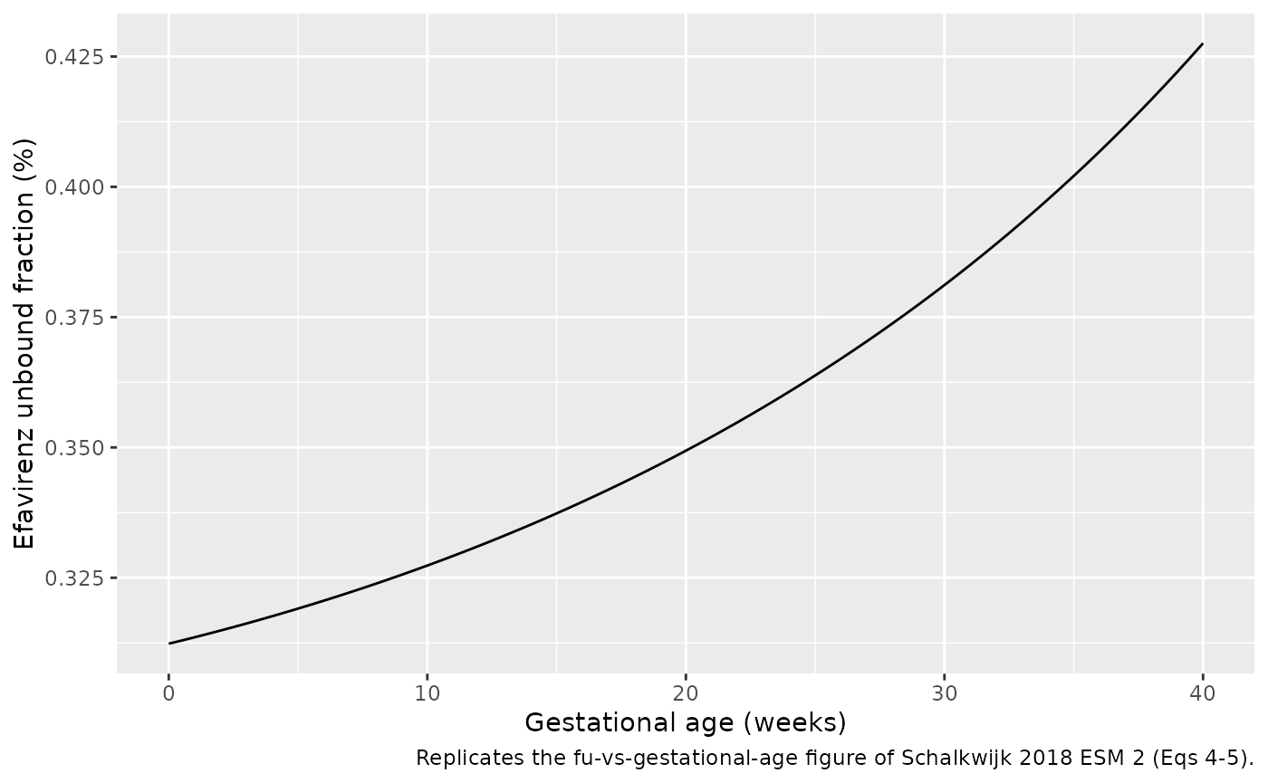
- falling serum albumin over gestation raises the unbound fraction
fu(Eqs 4-5), which raises the apparent hepatic clearance of a low-extraction drug; - falling haematocrit raises hepatic plasma flow (Eqs 3, 6);
- a dichotomous pregnancy effect shortens the mean absorption time and raises relative bioavailability by 16% (Table 2).
CYP2B6 metabolizer phenotype selects one of three intrinsic clearances.
Population
The model was developed on 1749 plasma samples from 247 women with HIV pooled from six studies (Studies 2-7 of Table 1). Study 1 (11 women, 219 samples) was held out for external evaluation; including it gives the 258 women and 1968 samples (774 during pregnancy) quoted in the Abstract. 142 women contributed samples both during pregnancy (second or third trimester; gestational age 21-39 weeks) and postpartum, and 116 only when not pregnant. Median body weight ranged from 53 to 83 kg across studies. Women were Black, Caucasian, Thai and Hispanic across the studies (Table 1). All but five women took efavirenz 600 mg once daily. CYP2B6 genotype was available only for Study 7 (18% of women: 10 poor, 25 intermediate, 26 extensive metabolizers).
The same information is available programmatically via
readModelDb("Schalkwijk_2018_efavirenz")()$population.
Source trace
Every ini() value carries an in-file comment pointing to
its source. Eqs 1-9 are not legible in the PDF text layer; they were
read from the MathML of the EuropePMC full-text XML of the same
article.
| Equation / parameter | Value | Source location |
|---|---|---|
lmtt (MAT, non-pregnant) |
log(2.12 h) | Table 2 |
lmtt_preg (MAT, pregnant) |
log(1.67 h) | Table 2 |
lfdepot |
fixed log(1) | Methods 2.3 |
e_preg_fdepot |
0.16 | Table 2, ‘F (%) relative to non-pregnant women’ = 116 |
lclint (EM) |
log(4580 L/h) | Table 2 |
lclint_im |
log(3340 L/h) | Table 2 |
lclint_pm |
log(1380 L/h) | Table 2 |
lvc |
log(133 L) | Table 2 |
lvp |
log(390 L) | Table 2 |
lq |
log(35 L/h) | Table 2 |
lqh (Qhep) |
fixed log(109 L/h) | Methods 2.2 |
lkd (kD) |
fixed log(2.05 uM) | Methods 2.2 |
e_wt_cl, e_wt_vc
|
fixed 0.75, 1 | Methods 2.3 (70 kg reference) |
etalclint |
0.0975 (32% CV) | Table 2 |
etalmtt |
0.177 (44% CV) | Table 2 |
etaiov_lfdepot_1..6 |
0.0560 (24% CV) | Table 2; Methods 2.3 (1-6 visits) |
propSd |
0.18 | Table 2 |
| Mixture frequencies PM / IM / EM | 14 / 36 / 50% (fixed) | Results paragraph 2 |
CLhep/F = Qhep,plasma * Eh |
n/a | Eq 1 |
Eh = CLint * fu / (Qhep,plasma + CLint * fu) |
n/a | Eq 2 |
Qhep,plasma = (1 - Ht) * Qhep |
n/a | Eq 3 |
fu = kD / (kD + [P]) |
n/a | Eq 4 |
[P] (uM) = (45.8 - 0.1775 GA - 0.0033 GA^2) / 0.07 |
n/a | Eq 5 |
Ht (%) = 39.1 - 0.0544 GA - 0.0021 GA^2 |
n/a | Eq 6 |
ktr = (n + 1) / MAT, n = 3 |
n/a | Eq 7; Fig 1 caption |
Cfree = fu * Ctot (model output Cu) |
n/a | Eq 9 |
Virtual cohort
Methods 2.7 describes the simulation cohort behind Table 3: body weight log-normal with geometric mean 62 kg (geometric SD 1.3), gestational age normal with mean 34 and SD 2.3 weeks for the third trimester, and 400 or 600 mg once daily to steady state, stratified by CYP2B6 phenotype. The paper used 500 subjects per phenotype; this vignette uses 150 per arm (12 arms).
set.seed(20180308)
rxode2::rxSetSeed(20180308)

n_per_arm <- 150
arms <- expand.grid(
  phenotype = c("PM", "IM", "EM"),
  dose_mg = c(600, 400),
  preg_state = c("Non-pregnant", "Pregnant"),
  stringsAsFactors = FALSE
)
arms$arm_id <- seq_len(nrow(arms))

obs_times <- 696 + c(0, 0.5, 1, 1.5, 2, 3, 4, 6, 8, 10, 12, 16, 20, 24)

make_arm <- function(a, n) {
  ids <- (a$arm_id - 1L) * n + seq_len(n)
  subj <- tibble(
    id = ids,
    WT = exp(rnorm(n, log(62), log(1.3))),
    PREG = as.integer(a$preg_state == "Pregnant"),
    EGA = if (a$preg_state == "Pregnant") rnorm(n, 34, 2.3) else 0,
    CYP2B6_PM = as.integer(a$phenotype == "PM"),
    CYP2B6_IM = as.integer(a$phenotype == "IM"),
    OCC = 1L,
    phenotype = a$phenotype,
    preg_state = a$preg_state,
    dose_mg = a$dose_mg,
    arm = paste(a$preg_state, paste(a$dose_mg, "mg"), a$phenotype, sep = " | ")
  )
  doses <- subj |>
    mutate(time = 0, amt = a$dose_mg, ii = 24, addl = 29, evid = 1L, cmt = "depot")
  obs <- subj |>
    tidyr::crossing(time = obs_times) |>
    mutate(amt = 0, ii = 0, addl = 0, evid = 0L, cmt = "central")
  bind_rows(doses, obs)
}

events <- bind_rows(lapply(seq_len(nrow(arms)), function(i) make_arm(arms[i, ], n_per_arm))) |>
  arrange(id, time, desc(evid))
stopifnot(!anyDuplicated(unique(events[, c("id", "time", "evid")])))
Simulation
mod <- readModelDb("Schalkwijk_2018_efavirenz")
sim <- rxode2::rxSolve(
  mod,
  events = events,
  keep = c("arm", "phenotype", "preg_state", "dose_mg")
) |>
  as.data.frame()
#> ℹ parameter labels from comments will be replaced by 'label()'
#> Warning: some etas defaulted to non-mu referenced, possible parsing error: etaiov_lfdepot_1, etaiov_lfdepot_2, etaiov_lfdepot_3, etaiov_lfdepot_4, etaiov_lfdepot_5, etaiov_lfdepot_6
#> as a work-around try putting the mu-referenced expression on a simple line
Typical-value check against Table 3
Table 3 reports cohort medians. For a log-normal clearance the median AUC24 is close to the typical-value AUC24, so a deterministic solve at the cohort’s typical covariates (62 kg, 34 weeks of gestation) is a sharp test of the structural model and of every value in Table 2.
mod_typ <- rxode2::zeroRe(mod)
#> ℹ parameter labels from comments will be replaced by 'label()'
#> Warning: some etas defaulted to non-mu referenced, possible parsing error: etaiov_lfdepot_1, etaiov_lfdepot_2, etaiov_lfdepot_3, etaiov_lfdepot_4, etaiov_lfdepot_5, etaiov_lfdepot_6
#> as a work-around try putting the mu-referenced expression on a simple line
#> Warning: some etas defaulted to non-mu referenced, possible parsing error: etaiov_lfdepot_1, etaiov_lfdepot_2, etaiov_lfdepot_3, etaiov_lfdepot_4, etaiov_lfdepot_5, etaiov_lfdepot_6
#> as a work-around try putting the mu-referenced expression on a simple line

typ_events <- arms |>
  mutate(
    id = arm_id,
    WT = 62,
    PREG = as.integer(preg_state == "Pregnant"),
    EGA = 34 * PREG,
    CYP2B6_PM = as.integer(phenotype == "PM"),
    CYP2B6_IM = as.integer(phenotype == "IM"),
    OCC = 1L
  )
typ_events <- bind_rows(
  typ_events |> mutate(time = 0, amt = dose_mg, ii = 24, addl = 29, evid = 1L, cmt = "depot"),
  typ_events |>
    tidyr::crossing(time = seq(696, 720, by = 0.1)) |>
    mutate(amt = 0, ii = 0, addl = 0, evid = 0L, cmt = "central")
) |>
  arrange(id, time, desc(evid))

typ <- rxode2::rxSolve(mod_typ, events = typ_events, keep = c("phenotype", "preg_state", "dose_mg")) |>
  as.data.frame()
#> ℹ omega/sigma items treated as zero: 'etalclint', 'etalmtt', 'etaiov_lfdepot_1', 'etaiov_lfdepot_2', 'etaiov_lfdepot_3', 'etaiov_lfdepot_4', 'etaiov_lfdepot_5', 'etaiov_lfdepot_6'
#> Warning: multi-subject simulation without without 'omega'

trap <- function(x, y) sum(diff(x) * (head(y, -1) + tail(y, -1)) / 2)
typ_sum <- typ |>
  group_by(id, phenotype, preg_state, dose_mg) |>
  summarise(
    auc24 = trap(time, Cc),
    c12 = Cc[which.min(abs(time - 708))],
    auc24_free = trap(time, Cu),
    c12_free = Cu[which.min(abs(time - 708))],
    .groups = "drop"
  )

published <- tibble::tribble(
  ~preg_state, ~dose_mg, ~phenotype, ~auc24_pub, ~c12_pub,
  "Non-pregnant", 600, "PM", 154, 6.1,
  "Non-pregnant", 600, "IM", 63, 2.4,
  "Non-pregnant", 600, "EM", 46, 1.7,
  "Non-pregnant", 400, "PM", 103, 4.1,
  "Non-pregnant", 400, "IM", 42, 1.6,
  "Non-pregnant", 400, "EM", 31, 1.1,
  "Pregnant", 600, "PM", 140, 5.4,
  "Pregnant", 600, "IM", 57, 2.1,
  "Pregnant", 600, "EM", 42, 1.4,
  "Pregnant", 400, "PM", 93, 3.9,
  "Pregnant", 400, "IM", 38, 1.4,
  "Pregnant", 400, "EM", 28, 1.0
)

typ_cmp <- typ_sum |>
  inner_join(published, by = c("preg_state", "dose_mg", "phenotype")) |>
  mutate(
    auc_pct = 100 * (auc24 - auc24_pub) / auc24_pub,
    c12_pct = 100 * (c12 - c12_pub) / c12_pub
  ) |>
  arrange(preg_state, desc(dose_mg), factor(phenotype, levels = c("PM", "IM", "EM")))

typ_cmp |>
  transmute(
    preg_state, dose_mg, phenotype,
    auc24 = round(auc24, 1), auc24_pub, auc_pct = round(auc_pct, 1),
    c12 = round(c12, 2), c12_pub, c12_pct = round(c12_pct, 1)
  ) |>
  rename(
    "Pregnancy state" = preg_state,
    "Dose (mg QD)" = dose_mg,
    "Phenotype" = phenotype,
    "AUC24 typical (mg*h/L)" = auc24,
    "AUC24 Table 3" = auc24_pub,
    "AUC24 % diff" = auc_pct,
    "C12 typical (mg/L)" = c12,
    "C12 Table 3" = c12_pub,
    "C12 % diff" = c12_pct
  ) |>
knitr::kable(caption = "Typical-value steady-state AUC24 and C12 (62 kg; 34 weeks gestation) vs Table 3 medians.")| Pregnancy state | Dose (mg QD) | Phenotype | AUC24 typical (mg*h/L) | AUC24 Table 3 | AUC24 % diff | C12 typical (mg/L) | C12 Table 3 | C12 % diff |
|---|---|---|---|---|---|---|---|---|
| Non-pregnant | 600 | PM | 151.8 | 154 | -1.4 | 6.10 | 6.1 | 0.0 |
| Non-pregnant | 600 | IM | 63.0 | 63 | 0.0 | 2.40 | 2.4 | -0.1 |
| Non-pregnant | 600 | EM | 45.9 | 46 | -0.1 | 1.69 | 1.7 | -0.7 |
| Non-pregnant | 400 | PM | 101.2 | 103 | -1.7 | 4.07 | 4.1 | -0.8 |
| Non-pregnant | 400 | IM | 42.0 | 42 | 0.0 | 1.60 | 1.6 | -0.1 |
| Non-pregnant | 400 | EM | 30.6 | 31 | -1.2 | 1.13 | 1.1 | 2.3 |
| Pregnant | 600 | PM | 138.8 | 140 | -0.9 | 5.48 | 5.4 | 1.4 |
| Pregnant | 600 | IM | 57.4 | 57 | 0.7 | 2.09 | 2.1 | -0.3 |
| Pregnant | 600 | EM | 41.9 | 42 | -0.3 | 1.46 | 1.4 | 4.1 |
| Pregnant | 400 | PM | 92.5 | 93 | -0.5 | 3.65 | 3.9 | -6.4 |
| Pregnant | 400 | IM | 38.3 | 38 | 0.7 | 1.40 | 1.4 | -0.3 |
| Pregnant | 400 | EM | 27.9 | 28 | -0.3 | 0.97 | 1.0 | -2.8 |
All twelve AUC24 values agree with Table 3 to within 2%. Eleven of twelve C12 values agree to within the rounding of the published one- or two-digit values. The exception is the poor-metabolizer, pregnant, 400 mg cell: Table 3 prints a C12 of 3.9 mg/L with an IQR of 2.7-4.7, while its own AUC24 (93 mg*h/L) is exactly two-thirds of the 600 mg cell (140), whose C12 is 5.4. Linear PK gives 5.4 x 2/3 = 3.6, which the model reproduces; the printed 3.9 sits off-centre in its own IQR and is treated as a typesetting slip (see Assumptions and deviations).
# Deterministic solve, so tight bounds are appropriate. A mis-transcribed
# CLint, volume, Qhep, kD or polynomial coefficient moves AUC24 by >5%.
stopifnot(
  all(abs(typ_cmp$auc_pct) < 3),
  all(abs(typ_cmp$c12_pct[!(typ_cmp$preg_state == "Pregnant" & typ_cmp$dose_mg == 400 &
    typ_cmp$phenotype == "PM")]) < 7)
)
Pregnancy ratios quoted in the Abstract and Results
ratio_tab <- typ_sum |>
  filter(dose_mg == 400) |>
  select(phenotype, preg_state, auc24, c12, auc24_free, c12_free) |>
  pivot_wider(names_from = preg_state, values_from = c(auc24, c12, auc24_free, c12_free)) |>
  transmute(
    phenotype,
    auc_total = `auc24_Pregnant` / `auc24_Non-pregnant`,
    c12_total = `c12_Pregnant` / `c12_Non-pregnant`,
    auc_free = `auc24_free_Pregnant` / `auc24_free_Non-pregnant`,
    c12_free = `c12_free_Pregnant` / `c12_free_Non-pregnant`
  )

ratio_tab |>
  mutate(across(-phenotype, \(x) round(x, 3))) |>
  rename(
    "Phenotype" = phenotype,
    "Total AUC24 (paper 0.91)" = auc_total,
    "Total C12 (paper 0.87)" = c12_total,
    "Free AUC24 (paper 1.15)" = auc_free,
    "Free C12 (paper 1.11)" = c12_free
  ) |>
knitr::kable(caption = "Pregnant / non-pregnant ratios, typical subject, 400 mg QD.")| Phenotype | Total AUC24 (paper 0.91) | Total C12 (paper 0.87) | Free AUC24 (paper 1.15) | Free C12 (paper 1.11) |
|---|---|---|---|---|
| PM | 0.914 | 0.898 | 1.164 | 1.143 |
| IM | 0.911 | 0.874 | 1.160 | 1.112 |
| EM | 0.911 | 0.863 | 1.160 | 1.099 |
fu_np <- mod_typ |>
  rxode2::rxSolve(events = typ_events |> filter(id == 1, evid == 0) |> slice(1)) |>
  as.data.frame() |>
  pull(fu)
#> ℹ omega/sigma items treated as zero: 'etalclint', 'etalmtt', 'etaiov_lfdepot_1', 'etaiov_lfdepot_2', 'etaiov_lfdepot_3', 'etaiov_lfdepot_4', 'etaiov_lfdepot_5', 'etaiov_lfdepot_6'

stopifnot(
  all(abs(ratio_tab$auc_total - 0.91) < 0.02),
  all(abs(ratio_tab$c12_total - 0.87) < 0.03),
  all(abs(ratio_tab$auc_free - 1.15) < 0.03),
  all(abs(ratio_tab$c12_free - 1.11) < 0.04),
  # Methods 2.7: 0.7 mg/L x non-pregnant fu = 0.002 mg/L free target
  abs(0.7 * fu_np - 0.002) < 0.0003
)
The model reproduces the Abstract’s 91% (total AUC24) and 87% (total C12) pregnant-to-non-pregnant ratios, and the Results’ 15% (free AUC24) and 11% (free C12) increases. The non-pregnant unbound fraction is 0.00312, so the 0.7 mg/L total target maps to the paper’s free target of 0.002 mg/L.
Unbound fraction over gestation (ESM 2 figure)
fu_ga <- tibble(EGA = seq(0, 40, by = 0.5)) |>
  mutate(
    alb = (45.8 - 0.1775 * EGA - 0.0033 * EGA^2) / 0.07,
    fu = 2.05 / (2.05 + alb)
  )
ggplot(fu_ga, aes(EGA, 100 * fu)) +
  geom_line() +
  labs(
    x = "Gestational age (weeks)", y = "Efavirenz unbound fraction (%)",
    caption = "Replicates the fu-vs-gestational-age figure of Schalkwijk 2018 ESM 2 (Eqs 4-5)."
  )
PKNCA validation against Table 3
The stochastic cohort includes IIV on CLint/F and MAT and inter-occasion variability on F (one occasion per subject).
sim_nca <- sim |>
  filter(!is.na(Cc)) |>
  select(id, time, Cc, arm)

dose_df <- events |>
  filter(evid == 1) |>
  distinct(id, arm, amt) |>
  mutate(time = 696)

conc_obj <- PKNCA::PKNCAconc(sim_nca, Cc ~ time | arm + id, concu = "mg/L", timeu = "h")
dose_obj <- PKNCA::PKNCAdose(dose_df, amt ~ time | arm + id, doseu = "mg")

intervals <- data.frame(start = 696, end = 720, auclast = TRUE, cmax = TRUE)
nca_res <- PKNCA::pk.nca(PKNCA::PKNCAdata(conc_obj, dose_obj, intervals = intervals))

ref_nca <- published |>
  transmute(
    arm = paste(preg_state, paste(dose_mg, "mg"), phenotype, sep = " | "),
    auclast = auc24_pub
  )

cmp <- nlmixr2lib::ncaComparisonTable(
  simulated = nca_res,
  reference = ref_nca,
  by = "arm",
  params = "auclast",
  units = c(auclast = "mg*h/L"),
  tolerance_pct = 20
)
knitr::kable(cmp, caption = "Simulated median steady-state AUC24 (PKNCA) vs Table 3 medians. * differs by >20%.")| NCA parameter | arm | Reference | Simulated | % diff |
|---|---|---|---|---|
| AUClast (mg*h/L) | Non-pregnant | 600 mg | PM | 154 | 147 | -4.4% |
| AUClast (mg*h/L) | Non-pregnant | 600 mg | IM | 63 | 58.6 | -7.0% |
| AUClast (mg*h/L) | Non-pregnant | 600 mg | EM | 46 | 42.9 | -6.7% |
| AUClast (mg*h/L) | Non-pregnant | 400 mg | PM | 103 | 96.9 | -6.0% |
| AUClast (mg*h/L) | Non-pregnant | 400 mg | IM | 42 | 42.2 | +0.5% |
| AUClast (mg*h/L) | Non-pregnant | 400 mg | EM | 31 | 29.2 | -5.7% |
| AUClast (mg*h/L) | Pregnant | 600 mg | PM | 140 | 140 | +0.2% |
| AUClast (mg*h/L) | Pregnant | 600 mg | IM | 57 | 52.6 | -7.7% |
| AUClast (mg*h/L) | Pregnant | 600 mg | EM | 42 | 41.2 | -2.0% |
| AUClast (mg*h/L) | Pregnant | 400 mg | PM | 93 | 93.1 | +0.1% |
| AUClast (mg*h/L) | Pregnant | 400 mg | IM | 38 | 37.4 | -1.5% |
| AUClast (mg*h/L) | Pregnant | 400 mg | EM | 28 | 27.1 | -3.2% |
sim_auc <- as.data.frame(nca_res$result) |>
  filter(PPTESTCD == "auclast") |>
  group_by(arm) |>
  summarise(auc_med = median(PPORRES), .groups = "drop") |>
  inner_join(ref_nca, by = "arm") |>
  mutate(pct = 100 * (auc_med - auclast) / auclast)

# Each cell is a median of 150 subjects with ~40% CV on AUC24, so its
# sampling SE is ~4%; the median over 12 cells has an SE of ~1.6%. One
# 16-thread render gave a median of -3.5% and a worst cell of -7.7%, all
# sampling noise (the analytic F * Dose / (fu * CLint) medians of the same
# subjects agree with PKNCA). The deterministic typical-value gate above
# carries the tight structural check.
stopifnot(
  nrow(sim_auc) == 12,
  abs(median(sim_auc$pct)) < 7,
  max(abs(sim_auc$pct)) < 15
)
Mid-dose concentrations and target attainment
c12_sim <- sim |>
  filter(time == 708) |>
  group_by(preg_state, dose_mg, phenotype) |>
  summarise(
    c12_med = median(Cc),
    below_1 = 100 * mean(Cc < 1),
    below_07 = 100 * mean(Cc < 0.7),
    .groups = "drop"
  )

pct_published <- tibble::tribble(
  ~preg_state, ~dose_mg, ~phenotype, ~below_1_pub, ~below_07_pub,
  "Non-pregnant", 600, "PM", 0, 0,
  "Non-pregnant", 600, "IM", 3, 0,
  "Non-pregnant", 600, "EM", 9, 2,
  "Non-pregnant", 400, "PM", 0, 0,
  "Non-pregnant", 400, "IM", 15, 4,
  "Non-pregnant", 400, "EM", 41, 14,
  "Pregnant", 600, "PM", 0, 0,
  "Pregnant", 600, "IM", 7, 1,
  "Pregnant", 600, "EM", 23, 5,
  "Pregnant", 400, "PM", 0, 0,
  "Pregnant", 400, "IM", 23, 8,
  "Pregnant", 400, "EM", 53, 26
)

c12_tab <- c12_sim |>
  inner_join(published, by = c("preg_state", "dose_mg", "phenotype")) |>
  inner_join(pct_published, by = c("preg_state", "dose_mg", "phenotype")) |>
  arrange(preg_state, desc(dose_mg), factor(phenotype, levels = c("PM", "IM", "EM")))

c12_tab |>
  transmute(
    preg_state, dose_mg, phenotype,
    c12_med = round(c12_med, 2), c12_pub,
    below_1 = round(below_1), below_1_pub,
    below_07 = round(below_07), below_07_pub
  ) |>
  rename(
    "Pregnancy state" = preg_state,
    "Dose (mg QD)" = dose_mg,
    "Phenotype" = phenotype,
    "C12 median (mg/L)" = c12_med,
    "C12 Table 3" = c12_pub,
    "% < 1 mg/L" = below_1,
    "% < 1 mg/L Table 3" = below_1_pub,
    "% < 0.7 mg/L" = below_07,
    "% < 0.7 mg/L Table 3" = below_07_pub
  ) |>
knitr::kable(caption = "Simulated C12 and target attainment vs Table 3.")| Pregnancy state | Dose (mg QD) | Phenotype | C12 median (mg/L) | C12 Table 3 | % < 1 mg/L | % < 1 mg/L Table 3 | % < 0.7 mg/L | % < 0.7 mg/L Table 3 |
|---|---|---|---|---|---|---|---|---|
| Non-pregnant | 600 | PM | 5.90 | 6.1 | 0 | 0 | 0 | 0 |
| Non-pregnant | 600 | IM | 2.20 | 2.4 | 5 | 3 | 0 | 0 |
| Non-pregnant | 600 | EM | 1.62 | 1.7 | 11 | 9 | 2 | 2 |
| Non-pregnant | 400 | PM | 3.94 | 4.1 | 0 | 0 | 0 | 0 |
| Non-pregnant | 400 | IM | 1.63 | 1.6 | 12 | 15 | 2 | 4 |
| Non-pregnant | 400 | EM | 1.09 | 1.1 | 41 | 41 | 19 | 14 |
| Pregnant | 600 | PM | 5.54 | 5.4 | 0 | 0 | 0 | 0 |
| Pregnant | 600 | IM | 1.92 | 2.1 | 9 | 7 | 3 | 1 |
| Pregnant | 600 | EM | 1.48 | 1.4 | 26 | 23 | 5 | 5 |
| Pregnant | 400 | PM | 3.73 | 3.9 | 0 | 0 | 0 | 0 |
| Pregnant | 400 | IM | 1.39 | 1.4 | 25 | 23 | 10 | 8 |
| Pregnant | 400 | EM | 0.94 | 1.0 | 57 | 53 | 26 | 26 |
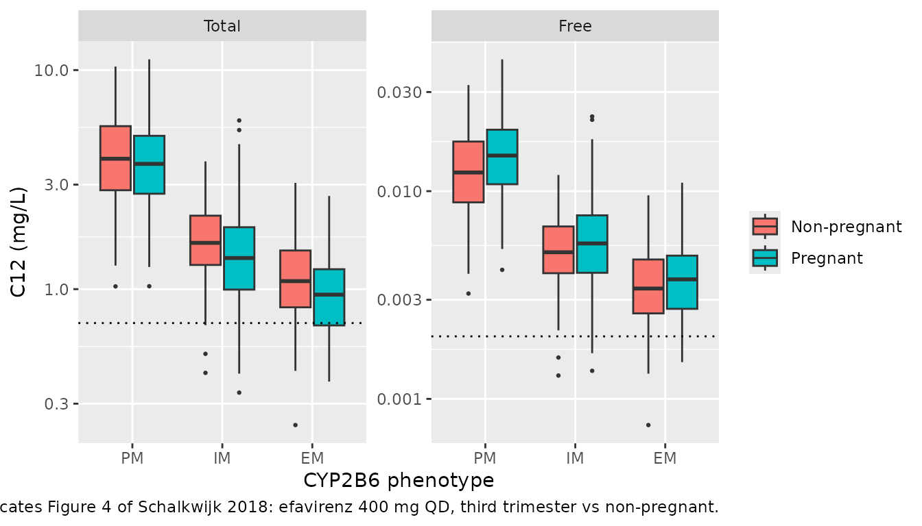
# The extensive-metabolizer 400 mg cells carry the paper's dose_mg-reduction
# argument (41% non-pregnant, 53% pregnant below 1 mg/L). A binomial
# proportion near 50% from 150 subjects has SE ~4 points.
em400 <- c12_tab |> filter(dose_mg == 400, phenotype == "EM")
stopifnot(all(abs(em400$below_1 - em400$below_1_pub) < 15))
Figure 4: total and free C12 at 400 mg
sim |>
  filter(time == 708, dose_mg == 400) |>
  select(id, preg_state, phenotype, Total = Cc, Free = Cu) |>
  pivot_longer(c(Total, Free), names_to = "measure", values_to = "conc") |>
  mutate(
    phenotype = factor(phenotype, levels = c("PM", "IM", "EM")),
    measure = factor(measure, levels = c("Total", "Free"))
  ) |>
  ggplot(aes(phenotype, conc, fill = preg_state)) +
  geom_boxplot(outlier.size = 0.5) +
  geom_hline(
    data = tibble(measure = factor(c("Total", "Free"), levels = c("Total", "Free")), target = c(0.7, 0.002)),
    aes(yintercept = target), linetype = "dotted"
  ) +
  facet_wrap(~measure, scales = "free_y") +
  scale_y_log10() +
  labs(
    x = "CYP2B6 phenotype", y = "C12 (mg/L)", fill = NULL,
    caption = "Replicates Figure 4 of Schalkwijk 2018: efavirenz 400 mg QD, third trimester vs non-pregnant."
  )
Steady-state profile by phenotype
sim |>
  filter(dose_mg == 400) |>
  mutate(tad = time - 696, phenotype = factor(phenotype, levels = c("PM", "IM", "EM"))) |>
  group_by(tad, preg_state, phenotype) |>
  summarise(
    Q05 = quantile(Cc, 0.05), Q50 = median(Cc), Q95 = quantile(Cc, 0.95),
    .groups = "drop"
  ) |>
  ggplot(aes(tad, Q50, colour = preg_state, fill = preg_state)) +
  geom_ribbon(aes(ymin = Q05, ymax = Q95), alpha = 0.15, colour = NA) +
  geom_line() +
  facet_wrap(~phenotype) +
  scale_y_log10() +
  labs(
    x = "Time after dose_mg (h)", y = "Total efavirenz (mg/L)", colour = NULL, fill = NULL,
    caption = "Simulated steady-state 400 mg QD profiles, median and 90% interval."
  )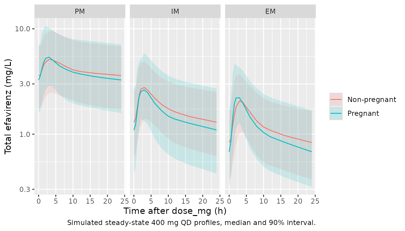
The paper’s Fig. 3 (prediction-corrected VPC against the observed data) cannot be reproduced without the individual data.
Assumptions and deviations
-
Algebraic well-stirred liver. Fig. 1 draws a
physical liver compartment with volume
Vh, butVhis not reported in the paper or either supplement. The maintainers encoded the liver as the paper’s own algebraic Eqs 1-2: systemic clearanceQhep,plasma * Ehfrom the central compartment, and a first-pass loss of the fractionEhon drug leaving the last transit compartment. Steady-state AUC does not depend onVh, and this encoding reproduces all twelve Table 3 AUC24 medians to within 2%. Both the first-pass factor and the allometric scaling ofQhepare needed; dropping either moves the predictions 10-20% from Table 3. -
Allometric scaling of Qhep. Methods 2.3 scales “all
flow parameters” to 70 kg with exponent 0.75. The maintainers applied
this to the literature hepatic blood flow
Qhep(109 L/h) as well as to CLint/F and Q/F; the Table 3 reproduction confirms it. -
Mixture model encoded as covariates. The paper
estimated CYP2B6 phenotype as a three-subpopulation mixture on CLint/F
with frequencies fixed to 14 / 36 / 50% (PM / IM / EM). The model file
takes the phenotype as the indicator columns
CYP2B6_PMandCYP2B6_IM(extensive metabolizer when both are 0). To simulate an unphenotyped population, draw the indicators with the paper’s 14 / 36 / 50% frequencies. -
Pooled poor-metabolizer level. The paper’s
poor-metabolizer subpopulation combines the ‘slow’ (516TT, or 516GT with
983TC) and ‘very slow’ (983CC) genotype classes listed in Methods 2.2.
The maintainers ratified the new canonical covariate
CYP2B6_PMfor this pooled level rather than reusing the strictCYP2B6_SM, whose 983CC subjects would otherwise fall to the extensive-metabolizer clearance. The four-class sentence in Methods 2.2 lists 983CC under both ‘slow’ and ‘very slow’; the three-level grouping actually fitted is unambiguous and is what is encoded. -
Two pregnancy covariates. Gestational age
(
EGA, weeks; 0 when not pregnant) drives the albumin and haematocrit polynomials; the binaryPREGcarries the MAT and F effects. SupplyPREG = 1exactly whenEGA > 0. Table 1 labels gestational age in “years”; the values and Methods 2.7 show the unit is weeks. -
Inter-occasion variability. IOV on F is encoded
with six occasion slots (Methods 2.3: one to six assessment visits per
woman), all sharing the estimated variance. This vignette sets
OCC = 1for every subject. -
%CV to variance. IIV and IOV were reported as %CV
and converted with
omega^2 = log(1 + CV^2). - C12 for poor metabolizers, pregnant, 400 mg. Table 3 prints 3.9 mg/L (IQR 2.7-4.7). Under the linear PK the paper assumes, this cell should be two-thirds of the 600 mg cell (5.4 mg/L), i.e. about 3.6 mg/L, as the printed AUC24 values are (93 vs 140). The model gives about 3.6 mg/L; the cell is excluded from the C12 gate.
- Simulation size. The paper simulated 500 women per phenotype; this vignette uses 150 per arm, so the stochastic medians and target-attainment percentages carry a few percentage points of sampling noise.
- No erratum to the article was found (checked 2026-10-16).