Eravacycline plasma and ELF (Ji 2025)
Source:vignettes/articles/Ji_2025_eravacycline.Rmd
Ji_2025_eravacycline.RmdModel and source
- Citation: Ji X-w, Mak WY, Xue F, Yang W-y, Kuan IH-S, Xiang X-q, Li Y, Zhu X. Population pharmacokinetics and pulmonary modeling of eravacycline and the determination of microbiological breakpoint and cutoff of PK/PD. Antimicrob Agents Chemother. 2025;69(3):e01065-24. doi:10.1128/aac.01065-24
- Description: Three-compartment intravenous population PK model for eravacycline in healthy adult volunteers (Ji 2025), fitted jointly to total plasma concentrations and to urea-corrected epithelial lining fluid (ELF) concentrations derived from bronchoalveolar lavage. ELF is not a kinetic compartment: under the authors’ quasi-equilibrium simplification the unbound ELF concentration is the unbound plasma concentration times an estimated ELF distribution ratio of 8.26. Unbound plasma concentration follows a fixed nonlinear power function of total concentration (Cu = 0.141 * Ctot^0.873, mg/L) carried from published binding data. Body weight enters allometrically (fixed exponents 0.75 on clearances and 1 on volumes, referenced to the 81.4 kg cohort median); no other covariate was retained.
- Article: https://doi.org/10.1128/aac.01065-24
Ji and colleagues re-analysed the Phase I bronchopulmonary-disposition study of intravenous eravacycline (TP-434-006) to build a population PK model of total plasma and epithelial lining fluid (ELF) concentrations, and used it in a Monte Carlo probability-of-target-attainment (PTA) analysis that proposes PK/PD cutoffs for four respiratory pathogens.
The final model (supplement Table S1, model 6) is a three-compartment
disposition model with allometric body-weight scaling. ELF was first
modelled as a kinetic compartment exchanging unbound drug with the
central compartment (rate constants k_cl and
k_lc, Figure 2 and supplement eq. 5-8), but with one
bronchoalveolar lavage (BAL) per subject those rate constants could not
be estimated. The authors therefore assumed quasi-equilibrium
(dA_ELF/dt = 0, supplement eq. 10), under which the two ELF
flux terms in the central ODE cancel exactly and the unbound ELF
concentration becomes
C_ELF = Ratio * C_u, C_u = 0.141 * C_tot^0.873 (mg/L)with Ratio = 8.26 estimated and the unbound plasma
concentration C_u obtained from total concentration through
a fixed power-law binding relationship taken from published binding data
(supplement eq. 1). The packaged model therefore has three ODE states
and two outputs: total plasma Cc and unbound ELF
Celf. The unbound plasma concentration is returned as
Cu.
Population
mod_fun <- readModelDb("Ji_2025_eravacycline")
str(rxode2::rxode(mod_fun)$population)
#> ℹ parameter labels from comments will be replaced by 'label()'
#> List of 14
#>  $ species       : chr "human"
#>  $ n_subjects    : num 20
#>  $ n_studies     : num 1
#>  $ age_range     : chr "19-47 years"
#>  $ age_median    : chr "27.5 years"
#>  $ weight_range  : chr "49.4-105 kg"
#>  $ weight_median : chr "81.4 kg"
#>  $ sex_female_pct: num 35
#>  $ race_ethnicity: Named num [1:2] 75 25
#>   ..- attr(*, "names")= chr [1:2] "Caucasian" "Other"
#>  $ disease_state : chr "healthy volunteers"
#>  $ dose_range    : chr "1 mg/kg IV over 1 h every 12 h for 7 doses"
#>  $ regions       : chr "United States (Phase I study TP-434-006, NCT01989949)"
#>  $ sampling      : chr "Plasma before and 1, 2, 4, 6 and 12 h after the last dose; one bronchoalveolar lavage per subject at 1, 2, 4, 6"| __truncated__
#>  $ notes         : chr "Ji 2025 Table 5 (demographics), Methods, and supplement section 'Human PK data collection'."
Twenty healthy volunteers (13 male, 7 female; 15 Caucasian) aged 19-47 years (median 27.5) and weighing 49.4-105 kg (median 81.4) received seven 1-hour infusions of eravacycline 1 mg/kg every 12 hours (Ji 2025 Table 5, supplement ‘Human PK data collection’). Plasma was sampled before and 1, 2, 4, 6 and 12 h after the last dose; each subject contributed one BAL at one of the same times.
Source trace
| Element | Value | Source |
|---|---|---|
| Structure: 3 compartments, quasi-equilibrium ELF | – | Supplement eq. 5-12; Table S1 model 6 |
lcl |
log(16.3 L/h) | Table 1 |
lvc |
log(3.88 L) | Table 1 |
lq |
log(33.9 L/h) | Table 1 (Q1) |
lvp |
log(39 L) | Table 1 (Vp1) |
lq2 |
log(23.5 L/h) | Table 1 (Q2) |
lvp2 |
log(122 L) | Table 1 (Vp2) |
lfelf |
log(8.26) | Table 1 (‘Ratio’); supplement eq. 12 |
fucoef, fupow
|
0.141, 0.873 (fixed) | Supplement eq. 1 and 9 |
e_wt_cl, e_wt_q, e_wt_q2
|
0.75 (fixed) | Table 1 footnote a |
e_wt_vc, e_wt_vp,
e_wt_vp2
|
1 (fixed) | Table 1 footnote a |
| Reference weight | 81.4 kg | Table 1 footnote a; Table 5 median |
etalcl |
log(1 + 0.136^2) | Table 1 IIV CL 13.6% |
etalvc |
log(1 + 1.16^2) | Table 1 IIV Vc 116% |
etalvp |
log(1 + 0.55^2) | Table 1 IIV Vp1 55% |
propSd |
0.0704 | Table 1 serum proportional error 7.04% |
addSd |
8.73 / 1000 mg/L | Table 1 serum additive error 8.73 (read as ng/mL) |
propSd_Celf |
0.423 | Table 1 BAL proportional error 42.3% |
Typical-value checks
Two deterministic checks run before any cohort is simulated. First, the quasi-equilibrium simplification leaves plasma disposition linear, so the steady-state total AUC over a day must equal the daily dose divided by clearance exactly. Second, the Methods quote an unbound plasma AUC of 1.5 mg*h/L for the approved 1 mg/kg q12h regimen (attributed to the bronchopulmonary study, reference 8 of the paper); the power-law binding plus the model’s clearance should land on it for a typical 81.4 kg subject.
mod <- rxode2::rxode(mod_fun)
#> ℹ parameter labels from comments will be replaced by 'label()'
mod_typ <- rxode2::zeroRe(mod)

wt_typ <- 81.4
ev_typ <- bind_rows(
  data.frame(
    id = 1L, time = seq(0, 156, by = 12), evid = 1L, amt = wt_typ,
    dur = 1, cmt = "central", dvid = NA_integer_
  ),
  data.frame(
    id = 1L, time = sort(unique(c(seq(0, 168, by = 1), seq(144, 168, by = 0.05)))),
    evid = 0L, amt = NA_real_, dur = NA_real_, cmt = "central", dvid = 1L
  )
) |>
  mutate(WT = wt_typ) |>
  arrange(id, time, desc(evid))

sim_typ <- as.data.frame(rxode2::rxSolve(mod_typ, ev_typ, useLinCmt = FALSE))
#> ℹ omega/sigma items treated as zero: 'etalcl', 'etalvc', 'etalvp'

trap <- function(t, y) sum(diff(t) * (head(y, -1) + tail(y, -1)) / 2)
day7 <- dplyr::filter(sim_typ, time >= 144)
typ <- data.frame(
  quantity = c("Total AUC24,ss (mg*h/L)", "Unbound plasma AUC24,ss (mg*h/L)", "Unbound ELF AUC24,ss (mg*h/L)"),
  simulated = c(trap(day7$time, day7$Cc), trap(day7$time, day7$Cu), trap(day7$time, day7$Celf)),
  expected = c(2 * wt_typ / 16.3, 1.5, NA)
)
knitr::kable(typ, digits = 3)| quantity | simulated | expected |
|---|---|---|
| Total AUC24,ss (mg*h/L) | 9.988 | 9.988 |
| Unbound plasma AUC24,ss (mg*h/L) | 1.536 | 1.500 |
| Unbound ELF AUC24,ss (mg*h/L) | 12.687 | NA |
stopifnot(
  # Closed form: AUC over a dosing day at steady state = daily dose / CL.
  abs(typ$simulated[1] / typ$expected[1] - 1) < 0.005,
  # Unbound plasma exposure quoted in the Methods for 1 mg/kg q12h.
  abs(typ$simulated[2] / typ$expected[2] - 1) < 0.10
)
The unbound ELF exposure of the typical subject is about 12.7 mgh/L, so at an MIC of 4 mg/L the typical subject sits at fAUC/MIC of about 3.2, just above the E. coli* target of 3. That is why the published PTA for the approved regimen at MIC 4 mg/L is neither 0% nor 100% (63.3%, supplement Table S5(A)).
Virtual cohort and regimens
The Monte Carlo analysis drew body weight from a uniform distribution between 50 and 100 kg (supplement ‘Dose optimization via Monte Carlo simulations’) and simulated the five regimens of Table 6 for seven days, computing the PTA from the unbound AUC at steady state. Here 200 virtual subjects are simulated per regimen; the same weights are reused across regimens.
rxode2::rxSetSeed(20250129)
n_per_arm <- 200
wt_cohort <- runif(n_per_arm, 50, 100)

regimens <- list(
  "Regimen 1" = list(times = seq(0, 156, by = 12), mgkg = rep(1, 14), dur = 1),
  "Regimen 2" = list(times = seq(0, 156, by = 12), mgkg = rep(1.5, 14), dur = 2),
  "Regimen 3" = list(times = seq(0, 144, by = 24), mgkg = rep(1.5, 7), dur = 2),
  "Regimen 4" = list(times = c(0, 12, seq(24, 144, by = 24)), mgkg = rep(1.5, 8), dur = 2),
  "Regimen 5" = list(times = seq(0, 156, by = 12), mgkg = c(1.5, 1.5, rep(1, 12)), dur = 2)
)

obs_times <- sort(unique(c(seq(0, 144, by = 2), seq(144, 168, by = 0.25))))

make_events <- function(k) {
  reg <- regimens[[k]]
  ids <- (k - 1L) * n_per_arm + seq_len(n_per_arm)
  doses <- tidyr::crossing(data.frame(id = ids, WT = wt_cohort), data.frame(time = reg$times, mgkg = reg$mgkg)) |>
    mutate(
      evid = 1L, amt = mgkg * WT, dur = reg$dur,
      cmt = "central", dvid = NA_integer_
    ) |>
    select(-mgkg)
  obs <- tidyr::crossing(data.frame(id = ids, WT = wt_cohort), data.frame(time = obs_times)) |>
    mutate(
      evid = 0L, amt = NA_real_, dur = NA_real_,
      cmt = "central", dvid = 1L
    )
  bind_rows(doses, obs) |>
    mutate(regimen = names(regimens)[k])
}

events <- bind_rows(lapply(seq_along(regimens), make_events)) |>
  arrange(id, time, desc(evid)) |>
  select(id, time, evid, amt, dur, cmt, dvid, WT, regimen)

sim <- as.data.frame(rxode2::rxSolve(
  mod, events,
  keep = c("regimen", "WT"), useLinCmt = FALSE
))
stopifnot(length(unique(sim$id)) == length(regimens) * n_per_arm)
Replicating Figure 5: concentrations after the last study dose
Figure 5 of the paper shows the plasma and BAL-derived ELF concentrations over the 12 h after the seventh (last) dose of 1 mg/kg q12h. The approved regimen (regimen 1) of the virtual cohort is plotted over the same post-dose window of its own final dosing interval (156-168 h).
last_int <- sim |>
  filter(regimen == "Regimen 1", time >= 156) |>
  mutate(tad = time - 156) |>
  select(id, tad, `Total plasma` = Cc, `Unbound ELF` = Celf) |>
  pivot_longer(c(`Total plasma`, `Unbound ELF`), names_to = "matrix", values_to = "conc") |>
  group_by(matrix, tad) |>
  summarise(
    p05 = quantile(conc, 0.05), p50 = median(conc), p95 = quantile(conc, 0.95),
    .groups = "drop"
  )

ggplot(last_int, aes(tad, p50)) +
  geom_ribbon(aes(ymin = p05, ymax = p95), alpha = 0.25, fill = "steelblue") +
  geom_line(colour = "steelblue4") +
  facet_wrap(~matrix, scales = "free_y") +
  scale_y_log10() +
  labs(x = "Time after last dose (h)", y = "Eravacycline (mg/L)")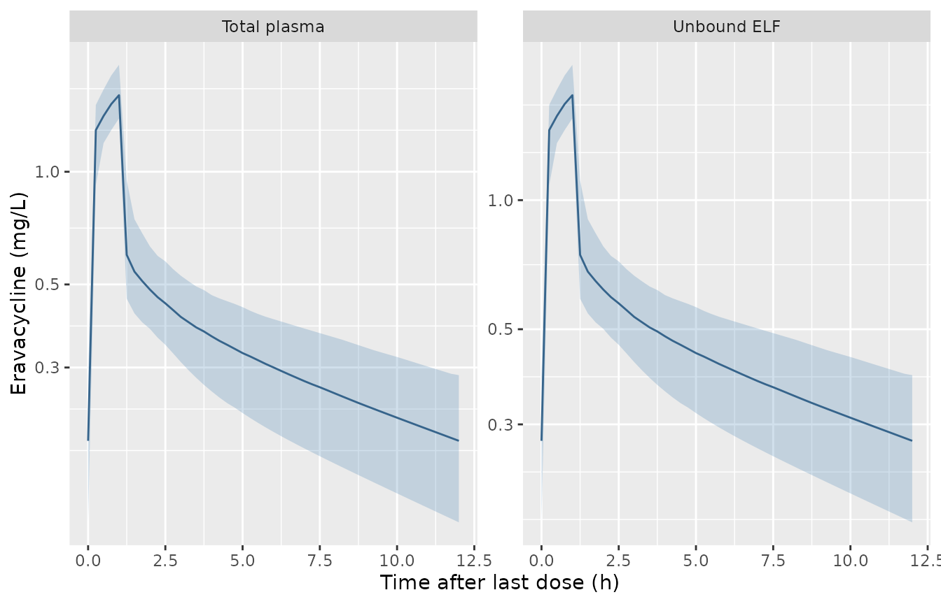
Replicates the layout of Figure 5 (plasma) and Figure S2 (ELF) of Ji 2025: median and 90% prediction interval after the last dose of 1 mg/kg q12h.
PKNCA: unbound exposure on day 7
The PK/PD index of the paper is the unbound AUC at steady state.
PKNCA computes it over the last 24 h of the seventh day (144-168 h) for
the unbound plasma (Cu) and unbound ELF (Celf)
concentrations, grouped by regimen.
dose_df <- events |>
  filter(evid == 1L) |>
  select(id, time, amt, regimen)

conc_cu <- sim |>
  filter(!is.na(Cu)) |>
  select(id, time, Cu, regimen)
conc_elf <- sim |>
  filter(!is.na(Celf)) |>
  select(id, time, Celf, regimen)

intervals <- data.frame(start = 144, end = 168, auclast = TRUE, cmax = TRUE)

nca_cu <- pk.nca(PKNCAdata(
  PKNCAconc(conc_cu, Cu ~ time | regimen + id),
  PKNCAdose(dose_df, amt ~ time | regimen + id),
  intervals = intervals
))
nca_elf <- pk.nca(PKNCAdata(
  PKNCAconc(conc_elf, Celf ~ time | regimen + id),
  PKNCAdose(dose_df, amt ~ time | regimen + id),
  intervals = intervals
))

nca_tab <- bind_rows(
  as.data.frame(nca_cu$result) |> mutate(matrix = "Unbound plasma"),
  as.data.frame(nca_elf$result) |> mutate(matrix = "Unbound ELF")
) |>
  group_by(matrix, regimen, PPTESTCD) |>
  summarise(median = median(PPORRES), .groups = "drop") |>
  pivot_wider(names_from = PPTESTCD, values_from = median)

nca_tab |>
  dplyr::rename(
    Matrix = matrix, Regimen = regimen,
    "Median fAUC144-168 (mg*h/L)" = auclast, "Median fCmax (mg/L)" = cmax
  ) |>
knitr::kable(digits = 3, caption = "Median day-7 unbound exposure by regimen.")| Matrix | Regimen | Median fAUC144-168 (mg*h/L) | Median fCmax (mg/L) |
|---|---|---|---|
| Unbound ELF | Regimen 1 | 12.421 | 1.757 |
| Unbound ELF | Regimen 2 | 18.058 | 1.746 |
| Unbound ELF | Regimen 3 | 9.390 | 1.543 |
| Unbound ELF | Regimen 4 | 9.716 | 1.573 |
| Unbound ELF | Regimen 5 | 12.483 | 1.246 |
| Unbound plasma | Regimen 1 | 1.504 | 0.213 |
| Unbound plasma | Regimen 2 | 2.186 | 0.211 |
| Unbound plasma | Regimen 3 | 1.137 | 0.187 |
| Unbound plasma | Regimen 4 | 1.176 | 0.190 |
| Unbound plasma | Regimen 5 | 1.511 | 0.151 |
The only steady-state NCA value the paper states is the unbound plasma AUC of 1.5 mg*h/L for the approved regimen (Methods, ‘Determination of PK/PD target values’).
published <- data.frame(regimen = "Regimen 1", auclast = 1.5)
simulated_r1 <- as.data.frame(nca_cu$result) |>
  filter(regimen == "Regimen 1")

cmp <- nlmixr2lib::ncaComparisonTable(
  simulated     = simulated_r1,
  reference     = published,
  by            = "regimen",
  params        = "auclast",
  units         = c(auclast = "mg*h/L"),
  tolerance_pct = 20
)
knitr::kable(cmp, caption = "Simulated vs. Ji 2025 Methods: unbound plasma AUC24,ss for 1 mg/kg q12h. * differs by >20%.")| NCA parameter | regimen | Reference | Simulated | % diff |
|---|---|---|---|---|
| AUClast (mg*h/L) | Regimen 1 | 1.5 | 1.5 | +0.2% |
Replicating supplement Table S5: probability of target attainment
PTA is the percentage of subjects whose unbound ELF AUC over day 7 divided by the MIC reaches the target (supplement eq. 17-18). The paper’s tables for E. coli (target 3) and for K. pneumoniae (targets 6 and 10) are reproduced below; the A. baumannii and S. aureus tables at target 10 are identical to the K. pneumoniae target-10 table over the shared MIC range.
fauc_elf <- as.data.frame(nca_elf$result) |>
  filter(PPTESTCD == "auclast") |>
  select(id, regimen, fauc = PPORRES)

mics <- c(0.004, 0.008, 0.016, 0.03, 0.06, 0.12, 0.25, 0.5, 1, 2, 4, 8, 16)
pta_sim <- tidyr::crossing(fauc_elf, mic = mics, target = c(3, 6, 10)) |>
  group_by(regimen, target, mic) |>
  summarise(pta = 100 * mean(fauc / mic >= target), .groups = "drop")

# Supplement Table S5(A) (target 3) and S5(B) (targets 10 and 6), MIC 0.03-16 mg/L.
pub_mic <- c(0.03, 0.06, 0.12, 0.25, 0.5, 1, 2, 4, 8, 16)
pub_t3 <- cbind(
  "Regimen 1" = c(100, 100, 100, 100, 100, 100, 100, 63.3, 0, 0),
  "Regimen 2" = c(100, 100, 100, 100, 100, 100, 100, 100, 1, 0),
  "Regimen 3" = c(100, 100, 100, 100, 100, 100, 99.9, 3.1, 0, 0),
  "Regimen 4" = c(100, 100, 100, 100, 100, 100, 100, 4.2, 0, 0),
  "Regimen 5" = c(100, 100, 100, 100, 100, 100, 100, 60.8, 0, 0)
)
pub_t10 <- cbind(
  "Regimen 1" = c(100, 100, 100, 100, 100, 95.1, 0, 0, 0, 0),
  "Regimen 2" = c(100, 100, 100, 100, 100, 100, 18.4, 0, 0, 0),
  "Regimen 3" = c(100, 100, 100, 100, 100, 38.2, 0, 0, 0, 0),
  "Regimen 4" = c(100, 100, 100, 100, 100, 38.2, 0, 0, 0, 0),
  "Regimen 5" = c(100, 100, 100, 100, 100, 95.9, 0, 0, 0, 0)
)
pub_t6 <- cbind(
  "Regimen 1" = c(100, 100, 100, 100, 100, 100, 63.3, 0, 0, 0),
  "Regimen 2" = c(100, 100, 100, 100, 100, 100, 100, 1, 0, 0),
  "Regimen 3" = c(100, 100, 100, 100, 100, 99.9, 3.1, 0, 0, 0),
  "Regimen 4" = c(100, 100, 100, 100, 100, 100, 4.2, 0, 0, 0),
  "Regimen 5" = c(100, 100, 100, 100, 100, 100, 60.8, 0, 0, 0)
)
to_long <- function(m, target) {
  as.data.frame(m) |>
    mutate(mic = pub_mic) |>
    pivot_longer(-mic, names_to = "regimen", values_to = "pta_pub") |>
    mutate(target = target)
}
pta_pub <- bind_rows(to_long(pub_t3, 3), to_long(pub_t6, 6), to_long(pub_t10, 10))

pta_cmp <- inner_join(pta_pub, pta_sim, by = c("regimen", "target", "mic"))

pta_cmp |>
  filter(mic >= 0.5, mic <= 8) |>
  mutate(cell = sprintf("%.1f / %.1f", pta_pub, pta)) |>
  select(target, mic, regimen, cell) |>
  pivot_wider(names_from = regimen, values_from = cell) |>
  dplyr::rename("fAUC/MIC target" = target, "MIC (mg/L)" = mic) |>
knitr::kable(caption = "PTA (%), published / simulated, supplement Table S5. MICs at or below 0.25 mg/L are 100 / 100 throughout and MIC 16 mg/L is 0 / 0.")| fAUC/MIC target | MIC (mg/L) | Regimen 1 | Regimen 2 | Regimen 3 | Regimen 4 | Regimen 5 |
|---|---|---|---|---|---|---|
| 3 | 0.5 | 100.0 / 100.0 | 100.0 / 100.0 | 100.0 / 100.0 | 100.0 / 100.0 | 100.0 / 100.0 |
| 3 | 1.0 | 100.0 / 100.0 | 100.0 / 100.0 | 100.0 / 100.0 | 100.0 / 100.0 | 100.0 / 100.0 |
| 3 | 2.0 | 100.0 / 100.0 | 100.0 / 100.0 | 99.9 / 100.0 | 100.0 / 100.0 | 100.0 / 100.0 |
| 3 | 4.0 | 63.3 / 57.5 | 100.0 / 100.0 | 3.1 / 2.5 | 4.2 / 7.0 | 60.8 / 64.0 |
| 3 | 8.0 | 0.0 / 0.0 | 1.0 / 0.5 | 0.0 / 0.0 | 0.0 / 0.0 | 0.0 / 0.0 |
| 6 | 0.5 | 100.0 / 100.0 | 100.0 / 100.0 | 100.0 / 100.0 | 100.0 / 100.0 | 100.0 / 100.0 |
| 6 | 1.0 | 100.0 / 100.0 | 100.0 / 100.0 | 99.9 / 100.0 | 100.0 / 100.0 | 100.0 / 100.0 |
| 6 | 2.0 | 63.3 / 57.5 | 100.0 / 100.0 | 3.1 / 2.5 | 4.2 / 7.0 | 60.8 / 64.0 |
| 6 | 4.0 | 0.0 / 0.0 | 1.0 / 0.5 | 0.0 / 0.0 | 0.0 / 0.0 | 0.0 / 0.0 |
| 6 | 8.0 | 0.0 / 0.0 | 0.0 / 0.0 | 0.0 / 0.0 | 0.0 / 0.0 | 0.0 / 0.0 |
| 10 | 0.5 | 100.0 / 100.0 | 100.0 / 100.0 | 100.0 / 100.0 | 100.0 / 100.0 | 100.0 / 100.0 |
| 10 | 1.0 | 95.1 / 94.0 | 100.0 / 100.0 | 38.2 / 29.0 | 38.2 / 42.5 | 95.9 / 97.0 |
| 10 | 2.0 | 0.0 / 0.0 | 18.4 / 25.0 | 0.0 / 0.0 | 0.0 / 0.0 | 0.0 / 0.0 |
| 10 | 4.0 | 0.0 / 0.0 | 0.0 / 0.0 | 0.0 / 0.0 | 0.0 / 0.0 | 0.0 / 0.0 |
| 10 | 8.0 | 0.0 / 0.0 | 0.0 / 0.0 | 0.0 / 0.0 | 0.0 / 0.0 | 0.0 / 0.0 |
# Cells where the published PTA is neither 0% nor 100% carry the information;
# the saturated cells agree trivially.
partial <- filter(pta_cmp, pta_pub > 0, pta_pub < 100)
stopifnot(
  # Structural: a wrong binding exponent, ELF ratio or unit reading shifts every
  # partial cell by tens of percentage points.
  abs(median(partial$pta - partial$pta_pub)) < 5,
  quantile(abs(partial$pta - partial$pta_pub), 0.9) < 15
)
pta_sim |>
  filter((target == 3) | (target == 6)) |>
  mutate(panel = ifelse(target == 3, "E. coli, fAUC/MIC = 3", "K. pneumoniae, fAUC/MIC = 6")) |>
  filter(mic >= 0.03) |>
  ggplot(aes(mic, pta, colour = regimen)) +
  geom_line() +
  geom_point() +
  geom_hline(yintercept = 90, linetype = "dashed") +
  scale_x_log10() +
  facet_wrap(~panel) +
  labs(x = "MIC (mg/L)", y = "PTA (%)", colour = NULL)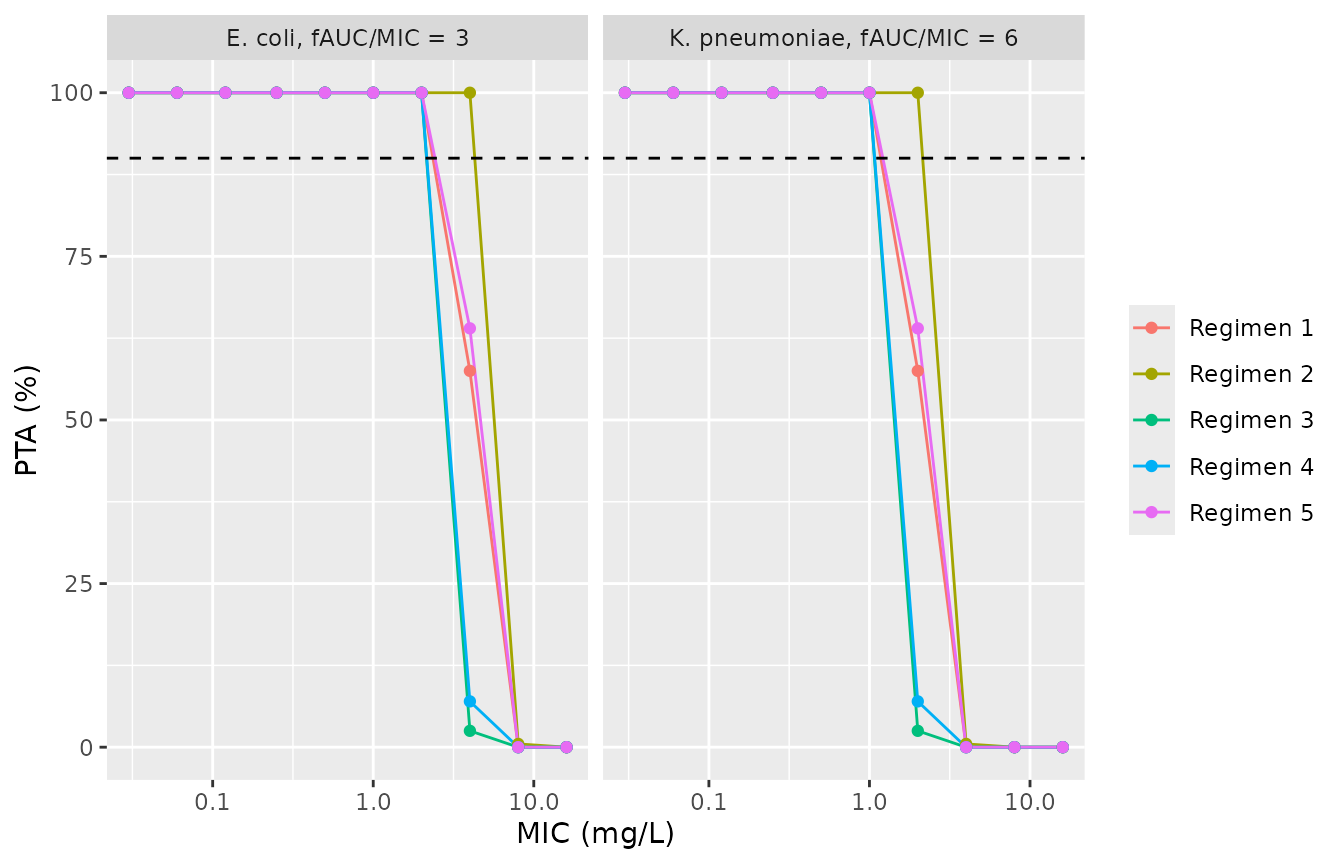
Replicates Figure 6A-B of Ji 2025: PTA against E. coli at fAUC/MIC = 3 and K. pneumoniae at fAUC/MIC = 6.
Replicating Table 4: cumulative fraction of response
The CFR weights the PTA at each MIC by the fraction of the 500 clinical isolates with that MIC (Table 2; supplement eq. 19).
mic_dist <- bind_rows(
  data.frame(bug = "E. coli", target = 3, mic = c(0.03, 0.06, 0.12, 0.25, 0.5, 1, 2), n = c(9, 67, 223, 142, 41, 12, 6)),
  data.frame(bug = "K. pneumoniae", target = 6, mic = c(0.03, 0.06, 0.12, 0.25, 0.5, 1, 2, 4, 8, 16), n = c(1, 8, 66, 157, 165, 44, 38, 14, 6, 1)),
  data.frame(bug = "A. baumannii", target = 10, mic = c(0.004, 0.008, 0.016, 0.03, 0.06, 0.12, 0.25, 0.5, 1, 2, 4), n = c(23, 14, 63, 134, 72, 47, 29, 84, 22, 8, 4)),
  data.frame(bug = "S. aureus", target = 10, mic = c(0.004, 0.008, 0.016, 0.03, 0.06, 0.12, 0.25, 0.5, 1), n = c(1, 52, 134, 121, 114, 33, 14, 19, 12))
)
stopifnot(all(tapply(mic_dist$n, mic_dist$bug, sum) == 500))

cfr_sim <- mic_dist |>
  inner_join(pta_sim, by = c("target", "mic"), relationship = "many-to-many") |>
  group_by(bug, regimen) |>
  summarise(cfr = sum(pta * n) / sum(n), .groups = "drop")

cfr_pub <- data.frame(
  bug = rep(c("E. coli", "K. pneumoniae", "A. baumannii", "S. aureus"), each = 5),
  regimen = rep(names(regimens), 4),
  cfr_pub = c(
    100, 100, 100, 100, 100,
    93.0, 95.8, 88.4, 88.5, 92.8,
    97.4, 97.9, 94.9, 94.9, 97.4,
    99.9, 100, 98.5, 98.5, 99.9
  )
)
cfr_cmp <- inner_join(cfr_pub, cfr_sim, by = c("bug", "regimen"))

cfr_cmp |>
  mutate(cell = sprintf("%.1f / %.1f", cfr_pub, cfr)) |>
  select(bug, regimen, cell) |>
  pivot_wider(names_from = regimen, values_from = cell) |>
  dplyr::rename(Bacterium = bug) |>
knitr::kable(caption = "CFR (%), published (Table 4) / simulated.")| Bacterium | Regimen 1 | Regimen 2 | Regimen 3 | Regimen 4 | Regimen 5 |
|---|---|---|---|---|---|
| E. coli | 100.0 / 100.0 | 100.0 / 100.0 | 100.0 / 100.0 | 100.0 / 100.0 | 100.0 / 100.0 |
| K. pneumoniae | 93.0 / 92.6 | 95.8 / 95.8 | 88.4 / 88.4 | 88.5 / 88.7 | 92.8 / 93.1 |
| A. baumannii | 97.4 / 97.3 | 97.9 / 98.0 | 94.9 / 94.5 | 94.9 / 95.1 | 97.4 / 97.5 |
| S. aureus | 99.9 / 99.9 | 100.0 / 100.0 | 98.5 / 98.3 | 98.5 / 98.6 | 99.9 / 99.9 |
Assumptions and deviations
-
IIV scale. Table 1 reports IIV as bare percentages
(13.6%, 116%, 55%) without saying whether they are the SD of eta or the
lognormal CV. They are encoded as lognormal CVs,
omega^2 = log(1 + CV^2). The PTA and CFR outputs cannot discriminate the two readings: they depend on clearance only, where the readings differ by 0.4%. - Additive residual error unit. Table 1 prints the serum additive error as 8.73 with no unit. It is read as ng/mL (8.73 / 1000 = 0.00873 mg/L): the bioanalytical calibration range is 5-500 ng/mL, and 8.73 mg/L would exceed the simulated peak concentrations. The rest of the model is in mg/L, which the binding equation requires (next item).
- Binding-equation units. Supplement eq. 1 does not state units. With total concentration in mg/L it gives an unbound fraction of about 19% at 0.1 mg/L falling to about 10.5% at 10 mg/L, consistent with eravacycline’s reported 79-90% plasma protein binding; the unbound plasma AUC it produces matches the 1.5 mg*h/L quoted in the Methods, and the resulting PTA table matches supplement Table S5 (above).
- Weight exponent. The Discussion states clearance scales with weight to the power 0.62 (Figure S1), whereas the model equations in Table 1 footnote a use 0.75. The 0.62 describes a post-hoc regression of individual clearance estimates on weight; the printed model equation (0.75) is encoded.
-
Figure 2 schematic. The schematic draws the ELF
rate constants
k_clandk_lc; the final model replaces them by the quasi-equilibrium ratio and they have no value. - BQL ELF samples. The Results report 5 of 20 BAL samples below the quantification limit, while the Discussion says four subjects (20%). The authors handled them with the M3 method; the packaged model carries no censoring, so simulated ELF concentrations are uncensored.
-
ELF is unbound. Observed ELF concentrations
(urea-corrected BAL) are treated as unbound drug because ELF protein
concentrations are low (supplement ‘ELF concentration determined from
BAL’);
Celfis thereforeRatio * Cu, notRatio * Cc. -
Table 2 MIC header. The MIC column headed
0.16in Table 2 lies between 0.008 and 0.03 and is read as 0.016 mg/L, the value used in Table S5(C-D). - Covariate screen. Age, albumin, ALT, creatinine clearance, total protein, red and white blood cell counts and sex were screened and none was retained (supplement Table S2); they are documented as excluded covariates.
- Virtual cohort. 200 subjects per regimen (the paper does not state its Monte Carlo size), so the simulated PTA carries a binomial error of a few percentage points at intermediate values.