Flunixin, florfenicol and penicillin G PBPK in cattle and swine (Chou 2022)
Source:vignettes/articles/Chou_2022_igpbpk.Rmd
Chou_2022_igpbpk.RmdModel and source
Chou 2022 builds an interactive generic physiologically based pharmacokinetic (igPBPK) platform for estimating withdrawal intervals (WDIs) of veterinary drugs in food animals. One flow-limited whole-body structure (plasma, liver, kidney, muscle, fat and a lumped rest of body, with a parallel metabolite submodel, a two-compartment gut and two-compartment intramuscular / subcutaneous injection sites) is calibrated separately for three drugs in two species. Six models are packaged, one per calibration, exactly as the authors fitted them:
models <- c(
  "Flunixin, cattle" = "Chou_2022_flunixin_cattle_pbpk",
  "Flunixin, swine" = "Chou_2022_flunixin_swine_pbpk",
  "Florfenicol, cattle" = "Chou_2022_florfenicol_cattle_pbpk",
  "Florfenicol, swine" = "Chou_2022_florfenicol_swine_pbpk",
  "Penicillin G, cattle" = "Chou_2022_penicillinG_cattle_pbpk",
  "Penicillin G, swine" = "Chou_2022_penicillinG_swine_pbpk"
)
uis <- lapply(models, function(m) rxode2::rxode2(readModelDb(m)))- Citation: Chou WC, Tell LA, Baynes RE, Davis JL, Maunsell FP, Riviere JE, Lin Z. An interactive generic physiologically based pharmacokinetic (igPBPK) modeling platform to predict drug withdrawal intervals in cattle and swine: a case study on flunixin, florfenicol, and penicillin G. Toxicol Sci. 2022;188(2):180-197. doi:10.1093/toxsci/kfac056. Model equations from Supplementary Equations S1-S16 and the authors’ deposited mrgsolve code (https://github.com/UFPBPK/FARAD-igPBPK, GenPBPK.R); physiology from Table 2; chemical-specific values from Tables 3 and 4 with fitted values at the precision of the deposited Fit_*.rds files; Monte Carlo distributions from Materials and Methods.
- Article: https://doi.org/10.1093/toxsci/kfac056
- Supplementary Data (equations S1-S22, tissue composition, dosing regimens): available with the article at the DOI above
- Authors’ code and data (mrgsolve model, fitted parameters, digitised observations): https://github.com/UFPBPK/FARAD-igPBPK
Each model takes body weight WT (kg) as its only
covariate. Doses are in mg and go into plasma
(intravenous), stomach (oral), depot +
depot2 (intramuscular; for flunixin depot
alone) or depot3 + depot4 (subcutaneous; for
flunixin depot3 alone). For the two-compartment injection
sites the same amount is dosed into both compartments and the model’s
bioavailability terms place the fraction Frac at the
fast-absorption site and 1 - Frac in the slow-release
depot. Concentrations are in mg/L (ug/g in tissue).
Population
No animals were dosed for this paper. Each drug-species model was calibrated by weighted least squares against mean concentration-time data collected from the Food Animal Residue Avoidance Databank (FARAD) Comparative Pharmacokinetic Database, taken from tables or digitised from figures (Chou 2022 Table 1), and evaluated against held-out studies. Data in dairy cows and lactating sows were excluded. The number of studies per model is:
pop <- bind_rows(lapply(names(uis), function(nm) {
  p <- uis[[nm]]$population
  data.frame(Model = nm, Studies = p$n_studies, Doses = p$dose_range)
}))
knitr::kable(pop)| Model | Studies | Doses |
|---|---|---|
| Flunixin, cattle | 7 | IV, IM or SC 2.2 mg/kg, single or once daily for 3-4 days |
| Flunixin, swine | 7 | IV 2-3 mg/kg, IM 2.2-2.4 mg/kg and oral 2.2-3.3 mg/kg, single or once daily for 3 days |
| Florfenicol, cattle | 11 | IV 2.2-50 mg/kg, IM 20 mg/kg, SC 40 mg/kg and oral 20-22 mg/kg, mostly single doses |
| Florfenicol, swine | 10 | IV, IM and oral 5-30 mg/kg, single or repeated for 2-5 days |
| Penicillin G, cattle | 5 | IM 6.9-65.4 mg/kg and SC 8.9-65.4 mg/kg procaine penicillin G, single or once daily for 3-5 days |
| Penicillin G, swine | 4 | IM 6.5-99 mg/kg and SC 99 mg/kg procaine penicillin G, single or once daily for 3-5 days |
Individual animal counts are not reported. The withdrawal-interval
simulations use 300 kg cattle and 92 kg swine (the authors’ code), with
body weight sampled normally (CV 20%). The full metadata is available as
readModelDb("Chou_2022_flunixin_cattle_pbpk")()$population.
Source trace
Every ini() value carries an in-file comment naming its
source. In summary:
| Element | Source |
|---|---|
| Two-compartment IM / SC injection sites | Supplementary Equations S1-S6; code Rim,
Rsiteim, ADOSEim
|
| Stomach and small intestine | Equations S7-S9; code RST, RSI (no stomach
uptake K0 in the code) |
Hepatic metabolism Rmet = KmetC*BW*AL
|
Equation S10; code Rmet
|
| Enterohepatic reabsorption and biliary return of parent and metabolite | Equations S11-S13; code RL, RSI
|
| Urinary excretion from kidney venous blood | Equation S14; code Rurine
|
| Flow-limited tissue mass balance | Equations S15-S16; code RK, RM,
RF, Rrest
|
Plasma state, CPlas = CPlas_free/Free, IV dose into
APlas_free
|
deposited code GenPBPK.R (not written out in the
supplement) |
| Flow and volume renormalisation | code $MAIN (sumQ, sumV) |
| Physiology (QCC, flow and volume fractions, Htc) | Table 2 |
| Chemical-specific parameters | Table 3 (cattle), Table 4 (swine); fitted values at the precision of
the deposited Fit_*.rds
|
| Gastric emptying GE = 0.182 /h | deposited code only |
| Monte Carlo coefficients of variation | Materials and Methods, ‘Establishment of a population PBPK model’; Table 2 SDs |
The typical values of all six models side by side (back-transformed;
fixed marks values not fitted by the authors):
ini_tab <- bind_rows(lapply(names(uis), function(nm) {
  d <- uis[[nm]]$iniDf
  d <- d[is.na(d$neta1) & is.na(d$err), ]
  d <- d[d$name != "propSd", ]
  val <- ifelse(startsWith(d$name, "l"), exp(d$est), d$est)
  data.frame(
    parameter = sub("_(5oh|floa|metab)$", "_met", d$name),
    model = nm,
    value = paste0(signif(val, 4), ifelse(d$fix, " (fixed)", ""))
  )
}))
ini_wide <- ini_tab |>
  pivot_wider(names_from = model, values_from = value, values_fill = "")
knitr::kable(ini_wide)| parameter | Flunixin, cattle | Flunixin, swine | Florfenicol, cattle | Florfenicol, swine | Penicillin G, cattle | Penicillin G, swine |
|---|---|---|---|---|---|---|
| lqcc | 5.45 (fixed) | 8.7 (fixed) | 5.45 (fixed) | 8.7 (fixed) | 5.45 (fixed) | 8.7 (fixed) |
| lfq_liver | 0.44 (fixed) | 0.273 (fixed) | 0.44 (fixed) | 0.273 (fixed) | 0.44 (fixed) | 0.273 (fixed) |
| lfq_kidney | 0.11 (fixed) | 0.114 (fixed) | 0.11 (fixed) | 0.114 (fixed) | 0.11 (fixed) | 0.114 (fixed) |
| lfq_muscle | 0.28 (fixed) | 0.342 (fixed) | 0.28 (fixed) | 0.342 (fixed) | 0.28 (fixed) | 0.342 (fixed) |
| lfq_fat | 0.08 (fixed) | 0.128 (fixed) | 0.08 (fixed) | 0.128 (fixed) | 0.08 (fixed) | 0.128 (fixed) |
| lfq_remainder | 0.09 (fixed) | 0.143 (fixed) | 0.09 (fixed) | 0.143 (fixed) | 0.09 (fixed) | 0.143 (fixed) |
| hct | 0.378 (fixed) | 0.412 (fixed) | 0.378 (fixed) | 0.412 (fixed) | 0.378 (fixed) | 0.412 (fixed) |
| fv_blood | 0.0399 (fixed) | 0.0412 (fixed) | 0.0399 (fixed) | 0.0412 (fixed) | 0.0399 (fixed) | 0.0412 (fixed) |
| fv_liver | 0.0122 (fixed) | 0.0204 (fixed) | 0.0122 (fixed) | 0.0204 (fixed) | 0.0122 (fixed) | 0.0204 (fixed) |
| fv_kidney | 0.0021 (fixed) | 0.0037 (fixed) | 0.0021 (fixed) | 0.0037 (fixed) | 0.0021 (fixed) | 0.0037 (fixed) |
| fv_muscle | 0.361 (fixed) | 0.3632 (fixed) | 0.361 (fixed) | 0.3632 (fixed) | 0.361 (fixed) | 0.3632 (fixed) |
| fv_fat | 0.1218 (fixed) | 0.1544 (fixed) | 0.1218 (fixed) | 0.1544 (fixed) | 0.1218 (fixed) | 0.1544 (fixed) |
| fv_remainder | 0.463 (fixed) | 0.4171 (fixed) | 0.463 (fixed) | 0.4171 (fixed) | 0.463 (fixed) | 0.4171 (fixed) |
| lka_im | 1 (fixed) | 1 (fixed) | 0.1618 (fixed) | 0.2108 | 0.1004 | 0.1036 |
| lka_sc | 0.4 (fixed) | 0.4 (fixed) | 0.128 (fixed) | 0.128 (fixed) | 0.04333 | 0.25 (fixed) |
| frac_im | 1 (fixed) | 1 (fixed) | 0.7089 | 0.5588 | 0.6517 | 0.5503 |
| frac_sc | 1 (fixed) | 1 (fixed) | 0.5639 | 0.5 (fixed) | 0.7559 | 0.5 (fixed) |
| lka | 0.4 (fixed) | 0.4 (fixed) | 1.91 (fixed) | 0.4 (fixed) | 1.91 (fixed) | 1.91 (fixed) |
| lkfec | 0.8134 | 0.5 (fixed) | 0.008762 | 0.1134 | 0.506 | 0.8133 |
| lkreab | 0.0121 | 0.004063 | 0.138 | 0.1683 | 0.0004338 | 0.01064 |
| lkmet | 0.004698 | 0.004257 | 0.2268 | 0.007457 | 0.2474 | 0.5945 |
| lfu | 0.1504 | 0.1275 | 0.7972 | 0.5897 | 0.6597 | 0.9565 |
| lfu_met | 0.007936 | 0.01 (fixed) | 0.71 (fixed) | 0.783 | 0.5 (fixed) | 0.634 (fixed) |
| lcl_bile | 0.5133 | 0.4012 | 0.1088 | 0.0308 | 0.6319 | 0.5212 |
| lcl_bile_met | 0.5798 | 0.03385 | 0.1564 | 0.0005983 | 0.1 (fixed) | 0.1 (fixed) |
| lcl_renal | 0.5002 | 0.2533 | 0.3151 | 0.4249 | 0.8252 | 1.541 |
| lcl_renal_met | 0.06843 | 0.007134 | 0.00152 | 0.01066 | 0.1 (fixed) | 0.1 (fixed) |
| lkp_liver | 2.196 | 2.301 | 1.98 | 0.3891 | 1.093 | 0.07405 |
| lkp_kidney | 3.381 | 6.998 | 0.9057 | 3.47 (fixed) | 1.98 | 1.426 |
| lkp_muscle | 0.4219 | 0.314 | 1.33 (fixed) | 1.3 (fixed) | 0.202 | 0.07886 |
| lkp_fat | 0.5601 | 0.6 (fixed) | 0.6072 | 0.1465 | 0.04 (fixed) | 0.249 (fixed) |
| lkp_remainder | 6.736 | 20.72 | 0.1221 | 1.165 | 7.994 | 0.4626 |
| lkp_liver_met | 3.11 (fixed) | 9.26 (fixed) | 7.596 | 14.8 | 10.52 (fixed) | 10.52 (fixed) |
| lkp_kidney_met | 4.598 | 4 (fixed) | 1.3 (fixed) | 5.989 | 4 (fixed) | 4 (fixed) |
| lkp_muscle_met | 2.96 (fixed) | 1.57 (fixed) | 0.9 (fixed) | 1.206 | 0.5 (fixed) | 0.5 (fixed) |
| lkp_remainder_met | 8.049 | 5 (fixed) | 0.09761 | 0.4933 | 8 (fixed) | 8 (fixed) |
| lkst | 0.182 (fixed) | 0.182 (fixed) | 0.182 (fixed) | 0.182 (fixed) | 0.182 (fixed) | 0.182 (fixed) |
| lkdiss_im | 0.0104 (fixed) | 0.02531 | 0.001036 | 0.007 (fixed) | ||
| lkdiss_sc | 0.005338 | 0.0054 (fixed) | 0.005 (fixed) | 0.005 (fixed) |
Here _met stands for the metabolite suffix:
_5oh (5-hydroxyflunixin), _floa (florfenicol
amine) or _metab (the unnamed penicillin G metabolites).
Rate constants lkreab (KehcC) and lkmet
(KmetC) and clearances lcl_* are per kg of body weight. The
values that depart from Tables 3 and 4, and why, are listed under Assumptions and deviations.
Known-answer check against the authors’ code
The authors deposited their mrgsolve model (GenPBPK.R).
The maintainers ran that code at the parameter values of these six
models, for each model’s FDA-label dosing regimen at the Monte Carlo
reference body weight, and recorded the concentrations below. The
packaged models must reproduce them; both sides use identical
parameters, so the difference is pure numerical error and a tight bound
is appropriate. In the authors’ code the intravenous dose is a 0.01 h
infusion, so the same is done here.
ref <- read.csv(text = "
model,time,Cc,Cliver,Ckidney,Cmuscle,Cfat,Cliver_met
flunixin_cattle,2,1.226465,2.552842,0.6371138,0.7766743,1.124748,0.252333
flunixin_cattle,24,0.05419192,0.09504076,0.02799181,0.02310643,0.03087084,0.009162087
flunixin_cattle,72,0.1168898,0.2050294,0.06037711,0.04983403,0.06657115,0.01981893
flunixin_cattle,168,0.02597646,0.04563712,0.01341761,0.01107331,0.01479053,0.00451684
flunixin_cattle,336,0.001912544,0.003403943,0.0009878816,0.0008151033,0.001088589,0.0003986561
flunixin_swine,2,1.318933,2.06956,3.18753,0.4852274,0.9944561,1.54397
flunixin_swine,24,0.04198555,0.0630502,0.09787952,0.01322758,0.02536991,0.1496104
flunixin_swine,72,0.02597187,0.03887123,0.0605444,0.00818058,0.01568486,0.08618912
flunixin_swine,168,0.01002775,0.01509005,0.02337614,0.003158473,0.006055714,0.04139794
flunixin_swine,336,0.001934584,0.002984505,0.004509727,0.0006093026,0.001168122,0.0152243
florfenicol_cattle,2,1.855422,2.43494,1.012728,2.35125,1.107178,28.07289
florfenicol_cattle,24,1.152048,2.39017,0.6289326,1.546899,0.7031442,70.00816
florfenicol_cattle,72,1.555775,3.232204,0.8493347,2.088046,0.9493232,94.80773
florfenicol_cattle,168,0.2645876,0.5425918,0.1444418,0.3539324,0.1611619,15.69939
florfenicol_cattle,336,0.03677871,0.07442747,0.02007779,0.04912105,0.02238333,2.12274
florfenicol_swine,2,3.368785,1.796175,6.753137,4.088849,0.4899038,0.4815058
florfenicol_swine,24,0.4033645,0.1655162,0.8123755,0.54764,0.05941271,2.766957
florfenicol_swine,72,0.4113388,0.1687898,0.8284352,0.5584621,0.06058716,6.781262
florfenicol_swine,168,0.0014596,0.0006584391,0.002934527,0.001908897,0.0002139774,5.668528
florfenicol_swine,336,0.0002362329,0.0001073777,0.000474878,0.000307967,3.461819e-05,0.9829525
penicillinG_cattle,2,0.3075396,0.2089425,0.1973019,0.06236005,0.01231269,4.21002
penicillinG_cattle,24,0.07437384,0.05732484,0.04771512,0.01508709,0.002977851,3.029427
penicillinG_cattle,72,0.1098062,0.09056919,0.07044511,0.02226176,0.004395929,6.395782
penicillinG_cattle,168,0.0336782,0.03309018,0.02160336,0.006810506,0.00134746,3.691955
penicillinG_cattle,336,0.01302391,0.01048009,0.008354013,0.002631349,0.0005209743,0.6887072
penicillinG_swine,2,0.4011939,0.02738793,0.2180032,0.03164852,0.09998842,0.4074324
penicillinG_swine,24,0.0676174,0.004710686,0.03674514,0.005336018,0.016876,0.4005359
penicillinG_swine,72,0.112746,0.007881215,0.0612667,0.008895583,0.02811936,0.8178036
penicillinG_swine,168,0.06826428,0.004761458,0.03709222,0.005383997,0.0170026,0.485455
penicillinG_swine,336,0.0206371,0.00143191,0.0112134,0.001627632,0.005139937,0.1134765
")
# Label (FDA-approved) regimens of Supplementary Table 8, as the authors
# simulated them (Figure_5_6.R in the deposited code).
label <- data.frame(
  key = c("flunixin_cattle", "flunixin_swine", "florfenicol_cattle", "florfenicol_cattle",
          "florfenicol_swine", "penicillinG_cattle", "penicillinG_swine"),
  scenario = c("IV 2.2 mg/kg q24h x3", "IM 2.2 mg/kg x1", "IM 20 mg/kg q48h x2",
               "SC 40 mg/kg x1", "oral 14 mg/kg q24h x5", "IM 6.5 mg/kg q24h x5",
               "IM 6.5 mg/kg q24h x5"),
  route = c("iv", "im", "im", "sc", "po", "im", "im"),
  dose = c(2.2, 2.2, 20, 40, 14, 6.5, 6.5),
  n = c(3, 1, 2, 1, 5, 5, 5),
  ii = c(24, 24, 48, 24, 24, 24, 24)
)
model_of <- function(key) models[[match(key, sub("Chou_2022_(.*)_pbpk", "\\1", models))]]

# Dosing rows for one animal. Two-compartment injection sites get the full
# amount in both compartments; the model's f() terms split it.
dose_rows <- function(route, amt, n, ii, dissolution) {
  t <- (seq_len(n) - 1) * ii
  cmts <- switch(route,
    iv = "plasma",
    po = "stomach",
    im = if (dissolution) c("depot", "depot2") else "depot",
    sc = if (dissolution) c("depot3", "depot4") else "depot3"
  )
  d <- expand.grid(time = t, cmt = cmts, stringsAsFactors = FALSE)
  d$amt <- amt
  d$rate <- if (route == "iv") amt / 0.01 else 0
  d$evid <- 1
  d
}

# Event table for a cohort: one block per animal, observations on `plasma`
# (a state; the algebraic outputs come back at every observation row).
cohort_events <- function(wt, route, dose, n, ii, dissolution, obs_times) {
  bind_rows(lapply(seq_along(wt), function(i) {
    dr <- dose_rows(route, dose * wt[i], n, ii, dissolution)
    ob <- data.frame(time = obs_times, cmt = "plasma", amt = 0, rate = 0, evid = 0)
    out <- bind_rows(dr, ob)
    out$id <- i
    out$WT <- wt[i]
    out
  })) |>
    arrange(id, time, desc(evid))
}

has_dissolution <- function(ui) "depot2" %in% ui$state
ka_check <- bind_rows(lapply(unique(ref$model), function(key) {
  ui <- uis[[match(model_of(key), models)]]
  lab <- label[match(key, label$key), ]
  wt <- ui$covariateData$WT$reference_value
  ev <- cohort_events(wt, lab$route, lab$dose, lab$n, lab$ii, has_dissolution(ui),
                      obs_times = c(2, 24, 72, 168, 336))
  sim <- rxode2::rxSolve(rxode2::zeroRe(ui), ev, atol = 1e-12, rtol = 1e-10,
                         maxsteps = 500000L, returnType = "data.frame")
  met_liver <- grep("^a_liver_", names(sim), value = TRUE)
  sim$Cliver_met <- sim[[met_liver]] / sim$v_liver
  r <- ref[ref$model == key, ]
  sim <- sim[match(r$time, sim$time), ]
  data.frame(model = key, time = r$time,
    max_rel_diff = apply(abs(as.matrix(sim[, names(r)[3:8]]) / as.matrix(r[, 3:8]) - 1), 1, max))
}))
knitr::kable(ka_check |> group_by(model) |> summarise(max_rel_diff = signif(max(max_rel_diff), 2)))| model | max_rel_diff |
|---|---|
| florfenicol_cattle | 4e-07 |
| florfenicol_swine | 2e-07 |
| flunixin_cattle | 4e-07 |
| flunixin_swine | 3e-07 |
| penicillinG_cattle | 4e-07 |
| penicillinG_swine | 4e-07 |
All six models reproduce the authors’ code to within the printed
precision of the reference values. Cliver_met is the
metabolite liver concentration (5-hydroxyflunixin, florfenicol amine, or
the unnamed penicillin G metabolites), so the metabolite submodels and
their molar coupling are checked too.
Mass balance
The authors’ code tracks amounts in mmol so that metabolism is mole-for-mole; the packaged models track mg and convert with the molecular-weight ratio. After a single dose every mole must still be somewhere: in the parent compartments, in the metabolite compartments, or excreted (biliary metabolite re-enters the gut as parent, so bile is not a sink).
# Molecular weights (g/mol) of parent and metabolite, Chou 2022 Table 3.
mw_tab <- list(flunixin = c(296.4, 312.4), florfenicol = c(358.2, 247.3),
               penicillinG = c(334, 334))
mb <- bind_rows(lapply(names(uis), function(nm) {
  ui <- uis[[nm]]
  mw <- mw_tab[[sub("Chou_2022_([A-Za-z]+)_.*", "\\1", models[[nm]])]]
  met <- sub("^plasma_", "", grep("^plasma_", ui$state, value = TRUE))
  wt <- ui$covariateData$WT$reference_value
  route <- if (has_dissolution(ui)) "im" else "sc"
  ev <- cohort_events(wt, route, 10, 1, 24, has_dissolution(ui), obs_times = c(24, 336))
  sim <- rxode2::rxSolve(rxode2::zeroRe(ui), ev, atol = 1e-12, rtol = 1e-10,
                         maxsteps = 500000L, returnType = "data.frame")
  parent <- setdiff(ui$state, c(grep(paste0("_", met, "$"), ui$state, value = TRUE), "a_metabolized"))
  metab <- grep(paste0("_", met, "$"), ui$state, value = TRUE)
  mol <- rowSums(sim[, parent]) / mw[1] + rowSums(sim[, metab]) / mw[2]
  data.frame(Model = nm, time = sim$time, recovered = mol / (10 * wt / mw[1]))
}))
knitr::kable(mb |> mutate(recovered = signif(recovered, 8)))| Model | time | recovered |
|---|---|---|
| Flunixin, cattle | 24 | 1 |
| Flunixin, cattle | 336 | 1 |
| Flunixin, swine | 24 | 1 |
| Flunixin, swine | 336 | 1 |
| Florfenicol, cattle | 24 | 1 |
| Florfenicol, cattle | 336 | 1 |
| Florfenicol, swine | 24 | 1 |
| Florfenicol, swine | 336 | 1 |
| Penicillin G, cattle | 24 | 1 |
| Penicillin G, cattle | 336 | 1 |
| Penicillin G, swine | 24 | 1 |
| Penicillin G, swine | 336 | 1 |
Withdrawal intervals: Monte Carlo replication of Figures 5 and 6 and Table 5
Sampling as the authors did
The authors’ Monte Carlo draws every parameter from a distribution
truncated at its 2.5th and 97.5th percentiles, and parameterises the
log-normal ones so that the arithmetic mean (not the median) equals the
tabulated value (logM = log(M / sqrt(1 + CV^2)) in the
deposited Pars.R). Neither feature can be expressed as an
ini() omega: the packaged models carry the tabulated value
as the typical value (median) and the authors’ CVs as fixed variances.
To reproduce the authors’ sampling exactly, the etas are drawn here
directly, truncated at |z| < 1.96 and shifted by
-omega^2/2 for the log-normal parameters, and passed to the
solver on a zeroRe() copy of the model. Body weight is
drawn from a normal distribution truncated at the same quantiles (mean
300 kg in cattle and 92 kg in swine, CV 20%).
rtrunc_z <- function(n) qnorm(runif(n, pnorm(-1.96), pnorm(1.96)))

draw_animals <- function(ui, n) {
  om <- diag(ui$omega)
  etas <- vapply(names(om), function(e) {
    sd <- sqrt(om[[e]])
    z <- rtrunc_z(n)
    # log-normal parameters (etal*) are mean-preserving, normal ones are not shifted
    if (startsWith(e, "etal")) -sd^2 / 2 + z * sd else z * sd
  }, numeric(n))
  if (n == 1) etas <- matrix(etas, nrow = 1, dimnames = list(NULL, names(om)))
  wt0 <- ui$covariateData$WT$reference_value
  data.frame(id = seq_len(n), WT = wt0 * (1 + 0.2 * rtrunc_z(n)), etas, check.names = FALSE)
}
Simulation
Each label regimen is simulated for 200 animals (the authors used 1000). The withdrawal interval is the first time after the last dose at which the 99th percentile of the tissue concentration falls to or below the tolerance, rounded up to whole days. For florfenicol the marker residue is florfenicol amine. Kidney uses the liver tolerance (Chou 2022 Methods).
rxode2::rxSetSeed(20220601)
set.seed(20220601)
n_animals <- 200

tolerances <- data.frame(
  key = c("flunixin_cattle", "flunixin_swine", "florfenicol_cattle", "florfenicol_swine",
          "penicillinG_cattle", "penicillinG_swine"),
  liver = c(0.125, 0.03, 3.7, 2.5, 0.05, 0.025),
  muscle = c(0.025, 0.025, 0.3, 0.2, 0.05, 0.025)
)

simulate_label <- function(i, theta_override = NULL) {
  lab <- label[i, ]
  ui <- uis[[match(model_of(lab$key), models)]]
  last <- (lab$n - 1) * lab$ii
  obs <- seq(0, last + 45 * 24, by = 3)
  draws <- draw_animals(ui, n_animals)
  if (!is.null(theta_override)) draws <- cbind(draws, as.data.frame(as.list(theta_override)))
  ev <- cohort_events(draws$WT, lab$route, lab$dose, lab$n, lab$ii, has_dissolution(ui), obs)
  sim <- suppressWarnings(rxode2::rxSolve(
    rxode2::zeroRe(ui), ev, params = draws[, names(draws) != "WT"],
    returnType = "data.frame", maxsteps = 500000L
  ))
  met <- if (startsWith(lab$key, "florfenicol")) "_floa" else ""
  tissue <- sim |>
    transmute(id, time,
      Liver = .data[[paste0("Cliver", met)]],
      Kidney = .data[[paste0("Ckidney", met)]],
      Muscle = .data[[paste0("Cmuscle", met)]]) |>
    pivot_longer(c(Liver, Kidney, Muscle), names_to = "tissue", values_to = "conc")
  tissue |>
    group_by(tissue, time) |>
    summarise(p01 = quantile(conc, 0.01), p50 = median(conc), p99 = quantile(conc, 0.99),
              .groups = "drop") |>
    mutate(scenario = lab$scenario, key = lab$key, last_dose = last)
}

mc <- bind_rows(lapply(seq_len(nrow(label)), simulate_label))
wdi_of <- function(d) {
  tol <- tolerances[match(d$key[1], tolerances$key), ]
  out <- d |>
    mutate(tol = ifelse(tissue == "Muscle", tol$muscle, tol$liver)) |>
    filter(time > last_dose, round(p99, 3) <= tol) |>
    group_by(tissue) |>
    summarise(wdi = ceiling(min(time - last_dose) / 24), .groups = "drop")
  out
}
wdi <- mc |>
  group_by(key, scenario) |>
  group_modify(~ wdi_of(mutate(.x, key = .y$key))) |>
  ungroup()

table5 <- data.frame(
  key = rep(label$key, each = 3),
  scenario = rep(label$scenario, each = 3),
  tissue = rep(c("Liver", "Kidney", "Muscle"), times = nrow(label)),
  table5 = c(7, 2, 8, 13, 14, 4, 26, 15, 28, 35, 19, 39, 16, 10, 16, 7, 3, 2, 1, 11, 1)
)
wdi_cmp <- wdi |>
  left_join(table5, by = c("key", "scenario", "tissue")) |>
  mutate(species = sub(".*_", "", key), drug = sub("_.*", "", key)) |>
  select(drug, species, scenario, tissue, wdi, table5)
wdi_cmp |>
  rename("Drug" = drug, "Species" = species, "Label regimen" = scenario, "Tissue" = tissue,
         "WDI, this model (days)" = wdi, "WDI, Chou 2022 Table 5 (days)" = table5) |>
knitr::kable()| Drug | Species | Label regimen | Tissue | WDI, this model (days) | WDI, Chou 2022 Table 5 (days) |
|---|---|---|---|---|---|
| florfenicol | cattle | IM 20 mg/kg q48h x2 | Kidney | 15 | 15 |
| florfenicol | cattle | IM 20 mg/kg q48h x2 | Liver | 25 | 26 |
| florfenicol | cattle | IM 20 mg/kg q48h x2 | Muscle | 27 | 28 |
| florfenicol | cattle | SC 40 mg/kg x1 | Kidney | 21 | 19 |
| florfenicol | cattle | SC 40 mg/kg x1 | Liver | 39 | 35 |
| florfenicol | cattle | SC 40 mg/kg x1 | Muscle | 40 | 39 |
| florfenicol | swine | oral 14 mg/kg q24h x5 | Kidney | 9 | 10 |
| florfenicol | swine | oral 14 mg/kg q24h x5 | Liver | 15 | 16 |
| florfenicol | swine | oral 14 mg/kg q24h x5 | Muscle | 16 | 16 |
| flunixin | cattle | IV 2.2 mg/kg q24h x3 | Kidney | 2 | 2 |
| flunixin | cattle | IV 2.2 mg/kg q24h x3 | Liver | 7 | 7 |
| flunixin | cattle | IV 2.2 mg/kg q24h x3 | Muscle | 8 | 8 |
| flunixin | swine | IM 2.2 mg/kg x1 | Kidney | 10 | 14 |
| flunixin | swine | IM 2.2 mg/kg x1 | Liver | 8 | 13 |
| flunixin | swine | IM 2.2 mg/kg x1 | Muscle | 2 | 4 |
| penicillinG | cattle | IM 6.5 mg/kg q24h x5 | Kidney | 3 | 3 |
| penicillinG | cattle | IM 6.5 mg/kg q24h x5 | Liver | 7 | 7 |
| penicillinG | cattle | IM 6.5 mg/kg q24h x5 | Muscle | 2 | 2 |
| penicillinG | swine | IM 6.5 mg/kg q24h x5 | Kidney | 11 | 11 |
| penicillinG | swine | IM 6.5 mg/kg q24h x5 | Liver | 1 | 1 |
| penicillinG | swine | IM 6.5 mg/kg q24h x5 | Muscle | 1 | 1 |
# The 99th percentile of 200 animals is an extreme order statistic whose
# value changes with the random stream, so the check is on the centre of the
# paired differences across all 21 tissue-regimen pairs, not on any one pair.
stopifnot(abs(median(wdi_cmp$wdi - wdi_cmp$table5)) <= 2)
The intervals agree with Table 5 to within the Monte Carlo noise of a 99th percentile estimated from 200 animals (rerunning the authors’ own code with different random seeds moves single intervals by about one day). Two systematic differences remain and are explained under Assumptions and deviations: Table 5 was generated with an earlier version of the authors’ code, and the swine flunixin model here uses the Table 4 absorption constants where that code used others.
plot_mc <- mc |>
  left_join(tolerances, by = "key") |>
  mutate(tol = ifelse(tissue == "Muscle", muscle, liver),
         day = (time - last_dose) / 24,
         panel = paste(scenario, sub("_", ", ", key), sep = "\n"),
         p01 = pmax(p01, 1e-6))
ggplot(plot_mc, aes(day, p50, colour = tissue)) +
  geom_line() +
  geom_line(aes(y = p99), linetype = 2) +
  geom_line(aes(y = p01), linetype = 3) +
  geom_hline(aes(yintercept = tol), linetype = 4, colour = "grey30") +
  scale_y_log10() +
  facet_wrap(~panel, scales = "free_y", ncol = 2) +
  labs(x = "Days after the last dose", y = "Tissue concentration (ug/g)",
       colour = "Tissue",
       title = "Replicates Figures 5 and 6 of Chou 2022",
       caption = "Median (solid), 1st and 99th percentiles (dotted, dashed); tolerance (dash-dot). Florfenicol: florfenicol amine.")
#> Warning in scale_y_log10(): log-10 transformation introduced infinite values.
#> log-10 transformation introduced infinite values.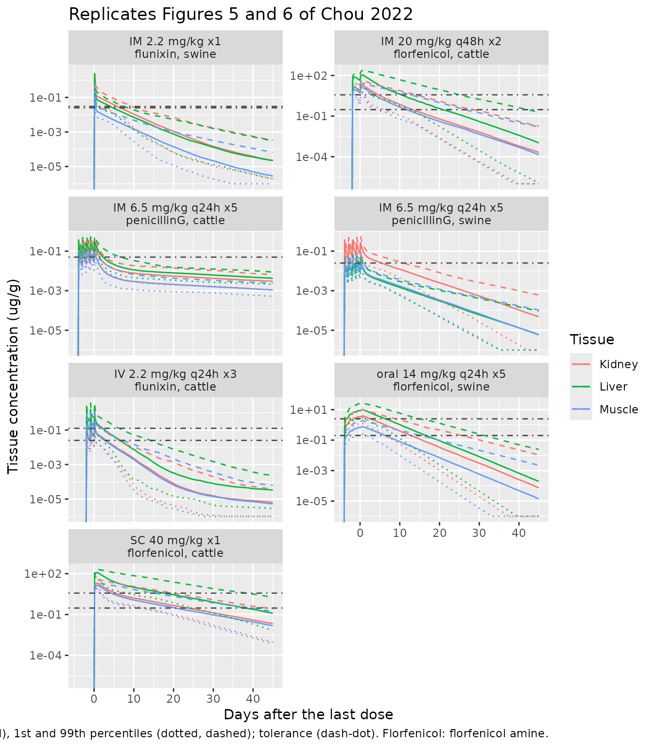
Effect of the swine flunixin absorption constants
For swine flunixin, Table 4 and the authors’ calibration script use Kim = 1 /h and Kabs = 0.4 /h (the values packaged here), but the figure and web-application code that produced Table 5 use Kim = 0.5 /h and Kabs = 1.9 /h. Rerunning the label regimen with the latter shows how much of the difference in the swine flunixin row they explain:
alt <- simulate_label(which(label$key == "flunixin_swine"),
                      theta_override = c(lka_im = log(0.5), lka = log(1.9)))
bind_rows(
  wdi_of(mc |> filter(key == "flunixin_swine")) |> mutate(values = "Table 4 (packaged)"),
  wdi_of(alt) |> mutate(values = "figure / app code")
) |>
  pivot_wider(names_from = values, values_from = wdi) |>
  rename("Tissue" = tissue) |>
knitr::kable()| Tissue | Table 4 (packaged) | figure / app code |
|---|---|---|
| Kidney | 10 | 14 |
| Liver | 8 | 12 |
| Muscle | 2 | 3 |
Noncompartmental analysis of the plasma profiles
Chou 2022 reports no noncompartmental parameters, so there is no published table to compare against; the typical-animal plasma profile after a single label dose is summarised with PKNCA as a reference for users.
nca_sims <- bind_rows(lapply(seq_len(nrow(label)), function(i) {
  lab <- label[i, ]
  ui <- uis[[match(model_of(lab$key), models)]]
  wt <- ui$covariateData$WT$reference_value
  ev <- cohort_events(wt, lab$route, lab$dose, 1, lab$ii, has_dissolution(ui),
                      obs_times = c(0, 0.25, 0.5, 1, 2, 4, 6, 8, 12, 24, 36, 48, 72, 96, 120, 168, 240, 336))
  sim <- rxode2::rxSolve(rxode2::zeroRe(ui), ev, returnType = "data.frame", maxsteps = 500000L)
  data.frame(treatment = paste(sub("_", ", ", lab$key), lab$route), id = 1L,
             time = sim$time, Cc = sim$Cc, dose = lab$dose * wt)
}))
conc_obj <- PKNCA::PKNCAconc(nca_sims |> filter(!is.na(Cc)), Cc ~ time | treatment + id)
dose_df <- nca_sims |> distinct(treatment, id, dose) |> mutate(time = 0)
dose_obj <- PKNCA::PKNCAdose(dose_df, dose ~ time | treatment + id)
intervals <- data.frame(start = 0, end = Inf, cmax = TRUE, tmax = TRUE, aucinf.obs = TRUE,
                        half.life = TRUE)
nca_res <- PKNCA::pk.nca(PKNCA::PKNCAdata(conc_obj, dose_obj, intervals = intervals))
as.data.frame(nca_res) |>
  filter(PPTESTCD %in% c("cmax", "tmax", "aucinf.obs", "half.life")) |>
  select(treatment, PPTESTCD, PPORRES) |>
  mutate(PPORRES = signif(PPORRES, 3)) |>
  pivot_wider(names_from = PPTESTCD, values_from = PPORRES) |>
  rename("Model and route" = treatment, "Cmax (mg/L)" = cmax, "Tmax (h)" = tmax,
         "AUC0-inf (mg*h/L)" = aucinf.obs, "t1/2 (h)" = half.life) |>
knitr::kable()| Model and route | Cmax (mg/L) | Tmax (h) | t1/2 (h) | AUC0-inf (mg*h/L) |
|---|---|---|---|---|
| florfenicol, cattle im | 1.880 | 4.00 | 62.4 | 97.20 |
| florfenicol, cattle sc | 2.600 | 4.00 | 120.0 | 193.00 |
| florfenicol, swine po | 4.080 | 4.00 | 66.4 | 54.00 |
| flunixin, cattle iv | 3.130 | 0.25 | 44.5 | 11.20 |
| flunixin, swine im | 2.450 | 0.25 | 70.3 | 11.20 |
| penicillinG, cattle im | 0.318 | 1.00 | 239.0 | 7.52 |
| penicillinG, swine im | 0.401 | 2.00 | 98.0 | 8.84 |
Assumptions and deviations
-
Equations from the deposited code. Supplementary
Equations S1-S16 give the structure only by example (the kidney stands
for every tissue) and do not write out the plasma compartment or the
metabolite submodel. The packaged ODEs are a line-by-line translation of
the authors’ mrgsolve code (
GenPBPK.R), which the known-answer check above reproduces exactly. -
Plasma state. As in the code, the intravenous dose
and the injection-site absorption enter the state the code calls
APlas_free, which carries the whole plasma mass balance, while the reported total plasma concentration isCPlas_free / Free, i.e.plasma / (v_plasma * fu). Tissue uptake isQ * CPlas * Free. This is kept exactly, because the fitted parameters were calibrated against it. -
Blood and plasma volume. Table 2 labels VPC as the
plasma volume fraction, but the code uses it as the blood volume and
takes
plasma = blood * (1 - Htc). The packaged models follow the code. - Swine flunixin Kim and Kabs. Table 4 and the calibration script give Kim = 1 /h and Kabs = 0.4 /h; the figure and web-application code (which produced Figures 5 and 6, Supplementary Figure 1 and Table 5) use 0.5 /h and 1.9 /h. The packaged model follows Table 4 and the calibration, under which the other swine flunixin parameters were fitted; the effect on the withdrawal intervals is shown above.
- Swine florfenicol Kabs. Table 4 prints 1.9 /h (Yang 2019), but both the calibration and the figure code use 0.4 /h, and with 0.4 /h the code reproduces the authors’ saved calibration predictions to within 0.01% (1.9 /h gives early oral concentrations about 20% higher). The packaged model uses 0.4 /h.
- Cattle florfenicol PM, PM1 and Kabs. The calibration script used the in silico PM = 1.53, PM1 = 0.27 and Kabs = 0.4 /h; Table 3 and the figure code give 1.33, 0.90 and 1.9 /h (1.91 in the code). The packaged model uses the Table 3 values.
- Penicillin G metabolite submodel. The paper says penicillin G metabolism is a first-order loss “without monitoring the distribution of its specific metabolites”, but the code runs the metabolite submodel for penicillin G too, with mrgsolve default parameters (PL1 10.52, PK1 4, PM1 0.5, PRest1 8, KurineC1 = KbileC1 = 0.1 L/h/kg, and fR1 0.5 in cattle and 0.634 in swine), and Supplementary Equation S13 returns its biliary excretion to the gut as parent. That recycling roughly doubles late liver and kidney residues in cattle, so it is kept, with the defaults the figure code used. None of these values is in the paper.
- Code-only values. The swine flunixin metabolite parameters (PL1 9.26, PK1 4, PM1 1.57, PRest1 5, fR1 0.01) and the gastric emptying constant GE = 0.182 /h for every model are in the code but not in the paper’s tables.
-
Precision. Fitted values are carried at the
precision of the deposited
Fit_*.rdsfiles; Tables 3 and 4 round or truncate them (for example cattle florfenicol fR 0.797 is printed 0.79 and swine florfenicol PL1 14.80 is printed 14.7). Literature values printed rounded in the tables use the code’s value where it is consistent with the rounding (cattle florfenicol Kim 0.1618, Ksc 0.128, Kdissim 0.0104; Kabs 1.91; swine florfenicol Kdisssc 0.0054; swine penicillin G PF 0.249). Molecular weights are those of Table 3 (the code uses 296.24 / 312.24 for flunixin and 358.21 / 247.28 for florfenicol); only their ratio enters the model and it differs by less than 0.02%. - Flunixin Frac. Flunixin has no dissolution step (Tables 3 and 4 leave Frac and Kdiss blank and the code sets Frac = 1), but the authors’ Monte Carlo still samples Frac (normal, CV 10%). The packaged flunixin models keep that as an IM / SC bioavailability factor with fixed variance.
-
Monte Carlo variability. The coefficients of
variation are the authors’ assumptions, fixed in
ini(): Table 2 SD / mean for physiology (including hematocrit, where the code instead uses CV 10%), 30% for the rest-of-body flow and volume, 20% for partition coefficients, 30% for rate constants and clearances and 10% for unbound fractions and Frac. Only the parameters the authors’ code samples carry an eta; for penicillin G that excludes the metabolite partition coefficients and clearances. The truncation at the 2.5th / 97.5th percentiles and the mean-preserving log-normal cannot be encoded inini(); the normal etas are clamped at +/-1.96 SD inmodel()so that a plainrxSolve()cannot produce a negative volume, and the vignette draws the etas itself to match the authors exactly. -
Table 5. The current deposited figure code measures
withdrawal intervals from the end of the last dosing interval and does
not reproduce Table 5. An earlier snapshot in the same repository
(
02032022_FARAD_Code, same parameters,set.seed(123)), which measures them from the time of the last dose and rounds up, regenerates Table 5 when the maintainers ran it: 38 of the 42 label and extralabel entries exactly and the other four (all swine) within one day. This vignette uses that definition. -
No residual-error model. The authors fitted by
weighted least squares and report none;
propSdis a fixed placeholder. - Tolerances. Kidney uses the liver tolerance (no kidney tolerances exist); penicillin G in swine uses the 0.025 ug/g minimum level of applicability because its US tolerance is zero (Chou 2022 Methods).