Cephalothin (Kuroda 2023)
Source:vignettes/articles/Kuroda_2023_cephalothin.Rmd
Kuroda_2023_cephalothin.RmdModel and source
- Citation: Kuroda T, Minamijima Y, Niwa H, Mita H, Tamura N, Fukuda K, Ohta M. (2023). Pharmacokinetic/pharmacodynamic analysis of cephalothin after intramuscular administration in Thoroughbred horses. Journal of Equine Science 34(4):111-114. doi:10.1294/jes.34.111.
- Description: Veterinary (Thoroughbred horse). Three-compartment population PK model for the first-generation cephalosporin cephalothin (CET) in Thoroughbred horses, fitted jointly to single-dose intramuscular (11 mg/kg bwt, 8 horses, this study) and single-dose intravenous (22 mg/kg bwt, 12 horses, Kuroda 2021 Equine Vet J 53:1239-1249) plasma data by nonlinear mixed-effects modelling in Phoenix WinNonlin 8.3. Absorption from the intramuscular site is first order (Kabs) with a bioavailability factor F; disposition is a central compartment (V1) connected to a rapidly equilibrating peripheral compartment (V2, distribution clearance CL2) and a slowly equilibrating peripheral compartment (V3, distribution clearance CL3), with elimination clearance CL from V1. Every structural parameter is reported per kilogram of body weight in Kuroda 2023 Table 1, so the model scales each of them linearly with WT (exponent 1 fixed); doses are therefore given in mg and concentrations come out in ug/mL. The unbound concentration Cu = fu * Cc (fu = 0.8, taken from Ambrose 2007 and used unchanged by Kuroda 2023) is the quantity that drives the paper’s PK/PD target, fT > MIC for 40% of the dosing interval, and its Monte Carlo probability of target attainment. Kuroda 2023 states that between-subject variability was described by an exponential model on the structural parameters but reports NO variance estimates anywhere (the Table 1 CV% column is bootstrap precision of the typical value, not BSV), so every eta is encoded as fixed(0) and the model simulates typical-value profiles unless the user supplies variances. The residual model is combined proportional plus additive; the additive component was estimated separately per route and the packaged value is the intramuscular one (see the addSd comment for the intravenous value).
- Article: J Equine Sci 34(4):111-114
- Companion intravenous study (pooled into the fit): Kuroda 2021, Equine Vet J 53:1239-1249
Cephalothin (CET) is a first-generation cephalosporin used as first-line treatment for equine gram-positive infections. Kuroda and colleagues gave a single 11 mg/kg intramuscular (IM) dose to eight Thoroughbred horses, pooled those data with a previously published 22 mg/kg intravenous (IV) dataset from 12 different horses, and fitted a single three-compartment nonlinear mixed-effects model with first-order IM absorption and a bioavailability factor. The model was then used in Monte Carlo simulations to pick an IM dosage regimen that attains the beta-lactam PK/PD target, free plasma concentration above the MIC (fT > MIC) for at least 40% of the dosing interval, in 90% of horses.
Population
Eight Thoroughbred horses (four stallions and four mares), four to nine years of age and weighing 490-570 kg, received 11 mg/kg bwt of cephalothin dissolved in 25 mL sterile physiological saline as a bolus IM injection (< 30 sec) into the right lateral neck. Plasma was sampled at 0, 5, 10, 20, 30 and 45 min and at 1, 2, 3, 4, 6, 8 and 12 hr, and assayed by LC-MS/MS with a limit of quantification of 0.1 ug/mL. Those data were aggregated with plasma concentrations from 12 different horses given 22 mg/kg IV (Kuroda 2021) and the pooled dataset was fitted in Phoenix WinNonlin 8.3; parameter precision came from a 50-replicate bootstrap. No neck pain, diarrhea or other side effects were observed.
The PK/PD targets are the MIC90 values of cephalothin against equine isolates of Streptococcus equi subsp. zooepidemicus (0.12 mg/L) and Staphylococcus aureus (0.5 mg/L).
The same information is available programmatically via the model’s
population metadata
(readModelDb("Kuroda_2023_cephalothin")()$population).
Source trace
The per-parameter origin is recorded as an in-file comment next to
each ini() entry in
inst/modeldb/specificDrugs/Kuroda_2023_cephalothin.R. The
table below collects them in one place for review. Kuroda 2023 Table 1
reports every primary structural parameter normalized to body weight, so
the model file stores the per-kilogram value and model()
multiplies by WT with an exponent of 1.
| Equation / parameter | Value as published | Value in ini()
|
Source location |
|---|---|---|---|
lvc |
V = 0.083 l/kg (CV% 8.1) |
log(0.083) L/kg |
Table 1, primary structural parameters |
lvp |
V2 = 0.060 l/kg (CV% 16.5) |
log(0.060) L/kg |
Table 1 |
lvp2 |
V3 = 0.054 l/kg (CV% 71.1) |
log(0.054) L/kg |
Table 1 |
lcl |
CL = 0.597 l/kg/hr (CV% 4.3) |
log(0.597) L/kg/hr |
Table 1 |
lq |
CL2 = 0.106 l/kg/hr (CV% 14.5) |
log(0.106) L/kg/hr |
Table 1 |
lq2 |
CL3 = 0.018 l/kg/hr (CV% 18.1) |
log(0.018) L/kg/hr |
Table 1 |
lka |
Kabs = 1.070 1/hr (CV% 24.6) |
log(1.070) 1/hr |
Table 1; cross-checks the secondary absorption half-life of 0.65 hr |
lfdepot |
F = 99.7% (CV% 9.8) | log(0.997) |
Table 1; repeated in the Results text |
fu |
free fraction = 0.8 | fixed(0.8) |
Methods para. 2, citing Ambrose 2007 (reference 1) |
propSd |
CMultStdev = 0.117 (CV% 9.5) | 0.117 |
Table 1, residual proportional component |
addSd |
stdev1 (IM) = 0.109 (CV% 50.0) |
0.109 ug/mL |
Table 1, residual additive component, IM arm |
all eta*
|
“BSV … described using an exponential model” (no variances reported) | fixed(0) |
Methods para. 2; see Errata |
d/dt(depot), f(depot)
|
Aa compartment, F and Kabs into V1 | n/a | Fig. 1 |
d/dt(central), d/dt(peripheral1),
d/dt(peripheral2)
|
V1 with Cl to V2 (Cl 12) and V3 (Cl 13), CL out of V1 | n/a | Fig. 1 and Methods para. 2 |
Cu <- fu * Cc |
free plasma concentration driving fT > MIC | n/a | Methods para. 2 |
Virtual cohort
Original observed data are not publicly available. The cohort below reproduces the eight-horse IM study: body weights are spread across the reported 490-570 kg range. Because Kuroda 2023 reports every structural parameter per kilogram and doses are given per kilogram, exposure is by construction independent of body weight; the cohort is simulated across the full weight range to demonstrate this rather than to generate spread.
obs_times <- sort(unique(c(seq(0, 12, by = 0.05), c(5, 10, 20, 30, 45) / 60)))

horses <- tibble(
  id = seq_len(8L),
  WT = round(seq(490, 570, length.out = 8))
)

events_im <- bind_rows(
  horses |>
    mutate(time = 0, amt = 11 * WT, evid = 1L, cmt = "depot"),
  horses |>
    crossing(time = obs_times) |>
    mutate(amt = NA_real_, evid = 0L, cmt = "central")
) |>
  arrange(id, time, desc(evid))

stopifnot(!anyDuplicated(events_im[, c("id", "time", "evid")]))
Simulation
All simulations use rxode2::zeroRe(). Kuroda 2023
reports no between-subject variance and no eta is therefore estimable
(see Errata), so the model produces typical-value profiles;
zeroRe() additionally suppresses the residual error so the
trajectories are the model’s deterministic predictions.
mod <- readModelDb("Kuroda_2023_cephalothin")
mod_typ <- rxode2::zeroRe(mod)

sim_im <- rxode2::rxSolve(
  mod_typ, events = events_im, returnType = "data.frame",
  # Tight solver tolerances: the weight-invariance gate below is at 1e-8.
  rtol = 1e-10, atol = 1e-12
) |>
  filter(!is.na(Cc))
#> ℹ omega/sigma items treated as zero: 'etalvc', 'etalvp', 'etalvp2', 'etalcl', 'etalq', 'etalq2', 'etalka', 'etalfdepot'
#> Warning: multi-subject simulation without without 'omega'

# Exposure is identical across the 490-570 kg range under mg/kg dosing.
stopifnot(
  diff(range(sim_im$Cc[sim_im$time == 1])) < 1e-8
)
Replicates Figure 2 of Kuroda 2023
Figure 2 of the paper is a semilogarithmic plot of the observed CET concentrations in the eight horses after the 11 mg/kg IM dose, over 0-15 hr on a 0.01-100 ug/mL axis. The typical-value curve below is plotted on the same axes. The observed between-horse spread in the published figure cannot be reproduced because no variance components were reported; the assay limit of quantification (0.1 ug/mL) is drawn for reference, since it explains why most published profiles end between 4 and 8 hr.
ggplot(sim_im |> filter(time > 0), aes(time, Cc, group = id)) +
  geom_line(linewidth = 0.7) +
  geom_hline(yintercept = 0.1, linetype = "dashed", colour = "grey40") +
  annotate(
    "text", x = 13, y = 0.115, label = "LOQ 0.1 ug/mL",
    hjust = 1, size = 3, colour = "grey30"
  ) +
  scale_y_log10(
    limits = c(0.01, 100),
    breaks = c(0.01, 0.1, 1, 10, 100),
    labels = c("0.01", "0.1", "1", "10", "100")
  ) +
  scale_x_continuous(limits = c(0, 15), breaks = seq(0, 15, by = 5)) +
  labs(x = "Time (hr)", y = "Observed concentration (ug/ml)") +
  theme_bw()
#> Warning: Removed 224 rows containing missing values or values outside the scale range
#> (`geom_line()`).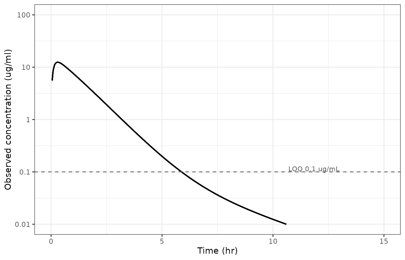
Replicates Figure 2 of Kuroda 2023: typical-value cephalothin plasma concentration after a single 11 mg/kg IM dose.
PKNCA validation
Kuroda 2023 reports no non-compartmental parameters, but Table 1 does report three model-derived secondary parameters for the pooled fit: the absorption half-life, the steady-state volume of distribution (Vss) and the mean residence time after IV dosing (MRT). Vss and MRT are exactly what NCA of a simulated IV profile returns, so they give a genuine numerical check on the packaged parameters. A 530 kg horse (the midpoint of the reported weight range) is used; because everything is per-kilogram, the choice does not affect the per-kilogram results.
wt_typ <- 530
nca_times <- seq(0, 36, by = 0.005)

solve_single <- function(amt_per_kg, route_cmt) {
  ev <- bind_rows(
    tibble(
      id = 1L, WT = wt_typ, time = 0,
      amt = amt_per_kg * wt_typ, evid = 1L, cmt = route_cmt
    ),
    tibble(
      id = 1L, WT = wt_typ, time = nca_times,
      amt = NA_real_, evid = 0L, cmt = "central"
    )
  ) |>
    arrange(time, desc(evid))
  rxode2::rxSolve(mod_typ, events = ev, returnType = "data.frame")
}

run_nca <- function(sim, amt_per_kg, treatment, route, intervals) {
  conc <- sim |>
    filter(!is.na(Cc)) |>
    transmute(id = 1L, time, Cc, treatment = treatment)
  dose <- tibble(
    id = 1L, time = 0, amt = amt_per_kg * wt_typ, treatment = treatment
  )
  conc_obj <- PKNCA::PKNCAconc(
    conc, Cc ~ time | treatment + id, concu = "ug/mL", timeu = "hr"
  )
  dose_obj <- PKNCA::PKNCAdose(
    dose, amt ~ time | treatment + id, doseu = "mg", route = route
  )
  as.data.frame(
    PKNCA::pk.nca(
      PKNCA::PKNCAdata(conc_obj, dose_obj, intervals = intervals)
    )$result
  )
}

sim_iv_nca <- solve_single(22, "central")
#> ℹ omega/sigma items treated as zero: 'etalvc', 'etalvp', 'etalvp2', 'etalcl', 'etalq', 'etalq2', 'etalka', 'etalfdepot'
sim_im_nca <- solve_single(11, "depot")
#> ℹ omega/sigma items treated as zero: 'etalvc', 'etalvp', 'etalvp2', 'etalcl', 'etalq', 'etalq2', 'etalka', 'etalfdepot'

nca_iv <- run_nca(
  sim_iv_nca, 22, "IV 22 mg/kg", "intravascular",
  data.frame(
    start = 0, end = Inf, cmax = TRUE, tmax = TRUE, aucinf.obs = TRUE,
    aumcinf.obs = TRUE, half.life = TRUE, cl.obs = TRUE,
    mrt.iv.obs = TRUE, vss.iv.obs = TRUE
  )
)
nca_im <- run_nca(
  sim_im_nca, 11, "IM 11 mg/kg", "extravascular",
  data.frame(
    start = 0, end = Inf, cmax = TRUE, tmax = TRUE, aucinf.obs = TRUE,
    half.life = TRUE
  )
)

pick <- function(res, code) res$PPORRES[res$PPTESTCD == code]
Comparison against the published secondary parameters
cl.obs, vss.iv.obs and
mrt.iv.obs from the simulated IV arm are compared against
Table 1. The two volume-derived rows are converted to a per-kilogram
basis to match the published units. For an intravenous dose CL/F is
simply CL.
sim_secondary <- tibble(
  PPTESTCD = c("cl.obs", "vss.iv.obs", "mrt.iv.obs"),
  PPORRES = c(
    pick(nca_iv, "cl.obs") / wt_typ,
    pick(nca_iv, "vss.iv.obs") / wt_typ,
    pick(nca_iv, "mrt.iv.obs")
  )
)

ref_secondary <- data.frame(
  cl.obs = 0.597,
  vss.iv.obs = 0.143,
  mrt.iv.obs = 0.24
)

tbl_secondary <- nlmixr2lib::ncaComparisonTable(
  sim_secondary, ref_secondary,
  units = c(
    cl.obs = "L/kg/hr", vss.iv.obs = "L/kg", mrt.iv.obs = "hr"
  )
)
knitr::kable(tbl_secondary, digits = 3)| NCA parameter | Reference | Simulated | % diff |
|---|---|---|---|
| CL/F (L/kg/hr) | 0.597 | 0.597 | -0.0% |
| MRT (IV) (hr) | 0.24 | 0.33 | +37.5%* |
| Vss (IV) (L/kg) | 0.143 | 0.197 | +37.8%* |
- differs from reference by more than ±20%.
Clearance is recovered exactly. Vss and MRT are both about 38% higher in the simulation than in Table 1, and the discrepancy has a single arithmetic explanation: the published Vss of 0.143 l/kg is exactly V1 + V2 (0.083 + 0.060), while the three-compartment model of Fig. 1 has Vss = V1 + V2 + V3 = 0.197 l/kg, and the published MRT of 0.24 hr is exactly 0.143 / 0.597 whereas the model gives 0.197 / 0.597 = 0.330 hr. The two published secondary values are internally consistent with each other but omit the third compartment. See Errata.
Absorption and bioavailability checks
Two further published quantities can be recomputed directly from the packaged parameters.
mod_ini <- rxode2::rxode(mod)$theta
ka_typ <- exp(unname(mod_ini["lka"]))

derived <- tibble(
  Quantity = c(
    "Absorption half-life (hr)",
    "Bioavailability F (fraction)"
  ),
  Published = c(0.65, 0.997),
  Simulated = c(
    log(2) / ka_typ,
    (pick(nca_im, "aucinf.obs") / (11 * wt_typ)) /
      (pick(nca_iv, "aucinf.obs") / (22 * wt_typ))
  )
) |>
  mutate(`% diff` = 100 * (Simulated - Published) / Published)

knitr::kable(derived, digits = 3)| Quantity | Published | Simulated | % diff |
|---|---|---|---|
| Absorption half-life (hr) | 0.650 | 0.648 | -0.338 |
| Bioavailability F (fraction) | 0.997 | 0.997 | -0.003 |
The bioavailability row is a round-trip check: it recovers
lfdepot from the ratio of dose-normalized AUCs of the
simulated IM and IV arms.
Simulated non-compartmental parameters
Kuroda 2023 reports no NCA table, so the following are given for reference rather than comparison. They are consistent with Fig. 2, where the peak lies between 10 and 30 ug/mL within the first hour and most profiles fall below the 0.1 ug/mL limit of quantification between 4 and 8 hr.
bind_rows(
  nca_im |> mutate(Treatment = "IM 11 mg/kg"),
  nca_iv |> mutate(Treatment = "IV 22 mg/kg")
) |>
  filter(PPTESTCD %in% c("cmax", "tmax", "aucinf.obs", "half.life")) |>
  transmute(
    Treatment,
    Parameter = nlmixr2lib::ncaParamLabel(
      PPTESTCD,
      units = c(
        cmax = "ug/mL", tmax = "hr", aucinf.obs = "hr*ug/mL",
        half.life = "hr"
      )
    ),
    Value = PPORRES
  ) |>
  pivot_wider(names_from = Treatment, values_from = Value) |>
knitr::kable(digits = 3)| Parameter | IM 11 mg/kg | IV 22 mg/kg |
|---|---|---|
| Cmax (ug/mL) | 12.467 | 265.060 |
| Tmax (hr) | 0.295 | 0.000 |
| t½ (hr) | 2.135 | 2.138 |
| AUC0-∞ (obs) (hr*ug/mL) | 18.370 | 36.851 |
PK/PD target attainment
The PK/PD index is fT > MIC, the time during which the
free plasma concentration Cu = fu * Cc exceeds the
MIC, and the target is 40% of the dosing interval. Kuroda 2023 evaluated
it over the 24 hr following the first administration.
Single-dose fT > MIC
dt <- 0.002
grid_24 <- seq(0, 24, by = dt)

solve_regimen <- function(tau) {
  n_extra <- if (is.null(tau)) 0L else floor((24 - 1e-9) / tau)
  dose <- tibble(
    id = 1L, WT = wt_typ, time = 0, amt = 11 * wt_typ,
    evid = 1L, cmt = "depot", ii = 0, addl = 0L
  )
  if (n_extra > 0L) {
    dose$ii <- tau
    dose$addl <- n_extra
  }
  ev <- bind_rows(
    dose,
    tibble(
      id = 1L, WT = wt_typ, time = grid_24, amt = NA_real_, evid = 0L,
      cmt = "central", ii = 0, addl = 0L
    )
  ) |>
    arrange(time, desc(evid))
  rxode2::rxSolve(mod_typ, events = ev, returnType = "data.frame") |>
    filter(!is.na(Cu))
}

single <- solve_regimen(NULL)
#> ℹ omega/sigma items treated as zero: 'etalvc', 'etalvp', 'etalvp2', 'etalcl', 'etalq', 'etalq2', 'etalka', 'etalfdepot'

tibble(
  Pathogen = c(
    "S. zooepidemicus (MIC90 0.12 mg/L)",
    "S. aureus (MIC90 0.5 mg/L)"
  ),
  `Published mean +/- SD (hr)` = c("7.1 +/- 2.6", "4.7 +/- 1.4"),
  `Typical horse (hr)` = c(
    sum(single$Cu > 0.12) * dt,
    sum(single$Cu > 0.5) * dt
  )
) |>
knitr::kable(digits = 2)| Pathogen | Published mean +/- SD (hr) | Typical horse (hr) |
|---|---|---|
| S. zooepidemicus (MIC90 0.12 mg/L) | 7.1 +/- 2.6 | 5.34 |
| S. aureus (MIC90 0.5 mg/L) | 4.7 +/- 1.4 | 3.69 |
The published values are arithmetic means over the eight study horses under a log-normal between-subject distribution, so they sit above the typical-value (median) prediction by construction; both simulated values fall well inside one published standard deviation.
Replicates Figure 3 of Kuroda 2023
Figure 3 plots the Monte Carlo probability of target attainment against MIC for 11 mg/kg IM given q6, q8, q12 and q24 hr, over the MIC grid 0.03-4 mg/L. With no between-subject variance available the Monte Carlo cohort collapses to a single typical horse, so the figure below plots the underlying quantity instead: the percentage of the 24 hr window during which the free concentration of the typical horse exceeds each MIC, against the 40% target. The typical horse corresponds to the 50th percentile of the published PTA curves, so the MIC at which it crosses 40% should sit above the published 90%-PTA breakpoint.
mic_grid <- c(0.03, 0.06, 0.12, 0.25, 0.5, 1, 2, 3, 4)
taus <- c(6, 8, 12, 24)

ft_mic <- lapply(taus, function(tau) {
  s <- solve_regimen(tau)
  tibble(
    tau = tau,
    mic = mic_grid,
    pct = vapply(
      mic_grid, function(m) 100 * mean(s$Cu > m), numeric(1)
    )
  )
}) |>
  bind_rows() |>
  mutate(regimen = factor(
    paste0("11 mg/kg q ", tau, " hr"),
    levels = paste0("11 mg/kg q ", taus, " hr")
  ))
#> ℹ omega/sigma items treated as zero: 'etalvc', 'etalvp', 'etalvp2', 'etalcl', 'etalq', 'etalq2', 'etalka', 'etalfdepot'
#> ℹ omega/sigma items treated as zero: 'etalvc', 'etalvp', 'etalvp2', 'etalcl', 'etalq', 'etalq2', 'etalka', 'etalfdepot'
#> ℹ omega/sigma items treated as zero: 'etalvc', 'etalvp', 'etalvp2', 'etalcl', 'etalq', 'etalq2', 'etalka', 'etalfdepot'
#> ℹ omega/sigma items treated as zero: 'etalvc', 'etalvp', 'etalvp2', 'etalcl', 'etalq', 'etalq2', 'etalka', 'etalfdepot'
ggplot(ft_mic, aes(mic, pct, colour = regimen, shape = regimen)) +
  geom_line() +
  geom_point(size = 2) +
  geom_hline(yintercept = 40, linewidth = 0.9) +
  geom_vline(xintercept = c(0.12, 0.5), linetype = "dotted") +
  scale_x_log10(breaks = mic_grid, labels = as.character(mic_grid)) +
  scale_y_continuous(limits = c(0, 100), breaks = seq(0, 100, by = 20)) +
  labs(
    x = "MIC (mg/l)", y = "fT > MIC over 24 hr (%)",
    colour = NULL, shape = NULL
  ) +
  theme_bw()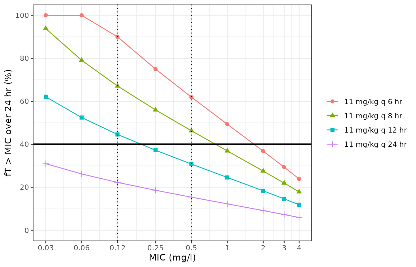
Replicates the structure of Figure 3 of Kuroda 2023: deterministic (typical-horse) fT > MIC over 24 hr versus MIC, with the 40% PK/PD target. Vertical dotted lines mark the published 90%-PTA breakpoints for q6 (0.5 mg/L) and q8 (0.12 mg/L).
published_bp <- c(`6` = 0.5, `8` = 0.12, `12` = 0.06, `24` = NA_real_)

ft_mic |>
  group_by(regimen, tau) |>
  summarise(
    typical = if (any(pct >= 40)) max(mic[pct >= 40]) else NA_real_,
    .groups = "drop"
  ) |>
  transmute(
    Regimen = regimen,
    `Published 90%-PTA breakpoint (mg/L)` = published_bp[as.character(tau)],
    `Typical-horse breakpoint (mg/L)` = typical,
    `Doubling dilutions higher` = log2(
      typical / published_bp[as.character(tau)]
    )
  ) |>
knitr::kable(digits = 2)| Regimen | Published 90%-PTA breakpoint (mg/L) | Typical-horse breakpoint (mg/L) | Doubling dilutions higher |
|---|---|---|---|
| 11 mg/kg q 6 hr | 0.50 | 1.00 | 1.00 |
| 11 mg/kg q 8 hr | 0.12 | 0.50 | 2.06 |
| 11 mg/kg q 12 hr | 0.06 | 0.12 | 1.00 |
| 11 mg/kg q 24 hr | NA | NA | NA |
The typical horse attains the target one to two doubling dilutions above the published 90%-PTA breakpoint for every regimen that has one, and the q24 hr regimen fails at every MIC on the grid, matching Fig. 3 where the q24 curve never approaches 90% (its highest plotted value is about 22% at 0.03 mg/L). This is the expected relationship between a median-horse threshold and a 90th-percentile requirement, and it reproduces the paper’s two headline conclusions: 11 mg/kg IM q 8 hr covers the S. zooepidemicus MIC90 of 0.12 mg/L and 11 mg/kg IM q 6 hr covers the S. aureus MIC90 of 0.5 mg/L.
Assumptions and deviations
Errata and source inconsistencies
-
No between-subject variance is reported. Kuroda
2023 Methods states that “the between-subject variability (BSV) was
described using an exponential model”, but no variance, standard
deviation or CV of any random effect appears anywhere in the paper. The
CV% column of Table 1 is the bootstrap precision of the typical
value (50 replicates), as the table title states, not BSV. Per the
standing policy for unreported IIV with structural values present, all
eight etas are encoded as
fixed(0)rather than invented. Consequences: the packaged model produces typical-value profiles only; the observed spread of Fig. 2 cannot be reproduced; and the Monte Carlo PTA of Fig. 3 collapses to the deterministic target-attainment analysis above. The paper also does not say which subset of the structural parameters carried BSV, so an eta placeholder is provided for all eight estimated structural parameters. - Published Vss and MRT omit the third compartment. Table 1’s secondary parameters, Vss = 0.143 l/kg and MRT = 0.24 hr, satisfy Vss = V1 + V2 = 0.083 + 0.060 and MRT = Vss / CL = 0.143 / 0.597, i.e. they are the two-compartment quantities. The three-compartment model of Fig. 1 gives Vss = V1 + V2 + V3 = 0.197 l/kg and MRT = 0.330 hr, which is what NCA of the simulated IV profile returns. The packaged model follows Fig. 1 and the primary structural parameters; the secondary parameters are not used to define it.
-
Residual additive-error units. Table 1 labels
stdev0 and stdev1 “ug/l”. The assay limit of quantification is 0.1 ug/ml
and Fig. 2 plots concentrations in ug/ml, so an additive residual SD of
0.109 ug/l would sit three orders of magnitude below the quantification
limit. The values are taken to be in the assay’s concentration units,
ug/mL (= mg/L), which is also what the Phoenix WinNonlin
stdevparameter carries. -
IM cohort size. Table 1’s caption says the IM data
came from “six horses”; the Abstract, the Methods and the Fig. 2 caption
all say eight, and Fig. 2 plots eight profiles. Eight is used in the
populationmetadata. -
Route-specific additive residual error. A single
proportional residual term (CMultStdev = 0.117) was estimated across
both routes, but the additive term was estimated separately: stdev0 =
0.008 for the IV data and stdev1 = 0.109 for the IM data. The packaged
addSdis the IM value, matching this model’s dosing route and the paper’s subject. To simulate the IV arm with the paper’s residual model, replaceaddSdwith 0.008. -
Bootstrap percentiles. Several of Table 1’s
2.5%/97.5% columns are internally inconsistent with their point
estimates (Kabs = 1.070 1/hr with a 0.001-0.002 interval; CL = 0.597
with a 97.5th percentile of 0.597; V3 = 0.054 with CV% 71.1 but a
0.039-0.057 interval). Only the typical values (medians) are used by the
model; the precision columns are recorded in the
ini()comments as published but are not relied on.
Modelling assumptions
-
Weight scaling. Table 1 reports every primary
structural parameter per kilogram, so
model()multiplies each volume and clearance byWTwith an exponent fixed at 1. This is a restatement of the published normalization, not an additional allometric assumption. Kabs (1/hr) and F are not weight-normalized in Table 1 and are used as-is. -
Free fraction.
fuis fixed at 0.8. Kuroda 2023 did not estimate it; the value is taken from Ambrose 2007 (reference 1 of the paper) exactly as the authors did. - Cohort size. The paper’s Monte Carlo simulations used 5,000 virtual horses. Because no variance components are available, additional simulated horses carry no information: under mg/kg dosing with per-kilogram parameters, exposure is identical for every body weight. The vignette therefore uses eight horses for the Fig. 2 replication (the study cohort size) and a single typical horse for the NCA and PK/PD calculations, well under the 200-per-arm vignette cap.
- Target attainment. The vertical breakpoint for the q12 hr regimen (0.06 mg/L) is read from the dotted lines of Fig. 3; the q6 and q8 hr breakpoints (0.5 and 0.12 mg/L) are stated in the Results and Discussion text.