Midazolam (Franken 2017)
Source:vignettes/articles/Franken_2017_midazolam.Rmd
Franken_2017_midazolam.RmdModel and source
- Citation: Franken LG, Masman AD, de Winter BCM, Baar FPM, Tibboel D, van Gelder T, Koch BCP, Mathot RAA. Hypoalbuminaemia and decreased midazolam clearance in terminally ill adult patients, an inflammatory effect? Br J Clin Pharmacol. 2017;83(8):1701-1712. doi:10.1111/bcp.13259.
- Description: Joint parent-metabolite population PK model for midazolam, its primary active metabolite 1-OH-midazolam (1-OH-M), and the secondary metabolite 1-OH-midazolam-glucuronide (1-OH-MG) in 45 terminally ill adult palliative-care patients (Franken 2017). Midazolam: one-compartment disposition with two parallel first-order absorption routes (oral and subcutaneous bolus) using route-specific absorption rate constants fixed from literature (Ka oral = 5.5 1/h, Ka SC = 10 1/h); oral bioavailability F is estimated and SC F assumed = 1. 1-OH-M: one compartment, central volume fixed equal to midazolam V, clearance estimated. 1-OH-MG: one compartment, clearance and volume estimated. All inter-compartment fluxes carry the parent / metabolite signal in midazolam-equivalent mass units (concentrations were adjusted to midazolam equivalents via molecular weight per Methods). Midazolam clearance depends on serum albumin (power form, reference 25 g/L) and 1-OH-MG clearance depends on eGFR (standard four-variable MDRD, power form, reference 104 mL/min/1.73 m^2). IIV on midazolam CL was correlated with oral F (rho fixed to unity per Results); other IIVs are independent. Residual variability is additive on log-transformed concentrations (LTBS) for all three analytes; a cross-output residual correlation noted in Methods is not encoded in this nlmixr2 port (see vignette Assumptions and deviations).
- Article: https://doi.org/10.1111/bcp.13259
Population
The published analysis included 45 terminally ill adult
palliative-care patients admitted to the Laurens Cadenza hospice
(Rotterdam, The Netherlands) over a two-year period. Median age 71 years
(range 43-93), 51.1% female, 91.1% Caucasian / 6.7% Afro-Caribbean /
2.2% Unknown; 97.8% had advanced malignancy as the primary diagnosis
(one patient with respiratory disease). Median duration of admittance
was 29 days (range 7-457). Patients received midazolam for insomnia or
palliative sedation per Dutch national guidelines, either orally up to
four times daily at 7.5 mg or subcutaneously (bolus or infusion) at
2.5-180 mg/day; the intravenous route was not used. Sparse plasma
sampling (median 2 samples per subject, range 1-10) yielded 139
quantifiable concentrations across midazolam, 1-OH-midazolam (1-OH-M),
and 1-OH-midazolam-glucuronide (1-OH-MG). Baseline blood-chemistry
medians at admission were albumin 25 g/L (range 13-39), creatinine 67
umol/L, eGFR by standard four-variable MDRD 104 mL/min/1.73 m^2 (range
6-328), CRP 92 mg/L. 37.8% used dexamethasone and 2.2% used phenytoin
during the observation window (concomitant CYP3A modulators). See
Franken 2017 Table 1 for the full baseline summary; the same information
is available programmatically via
readModelDb("Franken_2017_midazolam")$population.
Source trace
The per-parameter origin is recorded as an in-file comment next to
each ini() entry in
inst/modeldb/specificDrugs/Franken_2017_midazolam.R. The
table below collects them in one place.
| Equation / parameter | Final value | Source location |
|---|---|---|
lka_oral (Ka oral) |
5.5 1/h (FIXED) | Methods ‘Structural model’ (literature [16, 22, 25]) |
lka_sc (Ka SC) |
10 1/h (FIXED) | Methods ‘Structural model’ (literature [16, 22, 25]) |
lfdepot (F oral) |
0.279 | Table 2 Final |
lcl (midazolam CL at population median ALB) |
8.42 L/h | Table 2 Final |
lvc (midazolam V; also V_1OH-M) |
113 L | Table 2 Final (V_1OH-M assumed equal per Methods ‘Base model development’) |
lcl_1ohm (1-OH-M CL) |
45.4 L/h | Table 2 Final |
lcl_1ohmg (1-OH-MG CL at median eGFR) |
5.10 L/h | Table 2 Final |
lvc_1ohmg (1-OH-MG V) |
2.98 L | Table 2 Final (high RSE 71.5%) |
e_alb_cl (albumin power on midazolam CL) |
1.08 | Table 2 Final |
e_crcl_cl_1ohmg (eGFR power on 1-OH-MG CL) |
0.53 | Table 2 Final |
etalfdepot + etalcl block (rho = 1) |
50.6% / 49.0% CV, off-diagonal sqrt(var_F * var_CL) | Table 2 Final + Methods ‘Base model development’ (correlation 0.93 fixed to unity) |
etalvc (midazolam V) |
70.9% CV | Table 2 Final |
etalcl_1ohm (1-OH-M CL) |
60.5% CV | Table 2 Final |
etalcl_1ohmg (1-OH-MG CL) |
49.9% CV | Table 2 Final |
expSd (midazolam residual) |
sqrt(log(1 + 0.268^2)) | Table 2 Final (additive on log scale; CV% reported, converted to log-scale SD) |
expSd_1ohm (1-OH-M residual) |
sqrt(log(1 + 0.423^2)) | Table 2 Final |
expSd_1ohmg (1-OH-MG residual) |
sqrt(log(1 + 0.464^2)) | Table 2 Final |
| Equation: midazolam 1-cmt + 1-cmt 1-OH-M + 1-cmt 1-OH-MG cascade | n/a | Figure 2 schematic |
| Equation: power covariate forms theta = theta_pop * (cov / cov_m)^theta_cov | n/a | Methods Eq. 1 |
| Equation: ALB on midazolam CL, eGFR on 1-OH-MG CL | n/a | Methods Eqs. 4 and 5 |
Virtual cohort
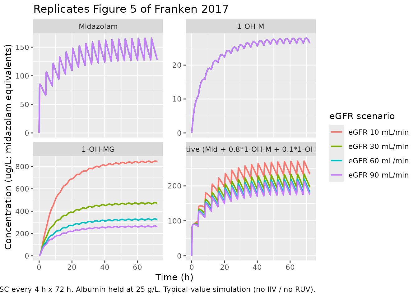
Original observed concentrations are not publicly available. The simulations below use typical-value virtual subjects whose covariates match the scenarios shown in Franken 2017 Figures 4 (albumin sweep) and 5 (eGFR sweep), plus the combined effect verification quoted in the Discussion / Simulations section.
set.seed(20170218)

# Figure 4 cohort: vary albumin at constant eGFR = 90 mL/min/1.73 m^2.
fig4 <- data.frame(
  id    = 1:3,
  ALB   = c(15, 25, 35),
  CRCL  = 90,
  scenario = factor(
    paste0("albumin ", c(15, 25, 35), " g/L"),
    levels = paste0("albumin ", c(15, 25, 35), " g/L")
  ),
  stringsAsFactors = FALSE
)

# Figure 5 cohort: vary eGFR at constant albumin = 25 g/L.
fig5 <- data.frame(
  id    = 4:7,
  CRCL  = c(10, 30, 60, 90),
  ALB   = 25,
  scenario = factor(
    paste0("eGFR ", c(10, 30, 60, 90), " mL/min"),
    levels = paste0("eGFR ", c(10, 30, 60, 90), " mL/min")
  ),
  stringsAsFactors = FALSE
)
Simulation
Both figures use the published simulation regimen from Methods
‘Simulations’: a 10 mg subcutaneous midazolam loading dose followed by 5
mg subcutaneously every 4 hours over 72 hours (six times daily). All
simulations zero out the between-subject variability and residual error
via rxode2::zeroRe() so that the resulting profiles are
typical-value replications of the published figures.
mod_typical <- readModelDb("Franken_2017_midazolam") |> rxode2::zeroRe()

build_events <- function(cov_df, obs_times, dose_events) {
  events_list <- lapply(seq_len(nrow(cov_df)), function(i) {
    row <- cov_df[i, , drop = FALSE]
    dose_rows <- dose_events |>
      dplyr::mutate(
        id       = row$id,
        ALB      = row$ALB,
        CRCL     = row$CRCL,
        scenario = as.character(row$scenario)
      )
    # One observation row per output per time point. Use the algebraic
    # observable name in cmt (rxode2 / rxUi auto-injects cmt(<observable>)
    # slots so the observable name is accepted on observation rows for
    # multi-output models).
    obs_rows <- tidyr::expand_grid(
      time = obs_times,
      cmt  = c("Cc", "Cc_1ohm", "Cc_1ohmg")
    ) |>
      dplyr::mutate(
        id       = row$id,
        amt      = NA_real_,
        rate     = NA_real_,
        evid     = 0L,
        ALB      = row$ALB,
        CRCL     = row$CRCL,
        scenario = as.character(row$scenario)
      )
    dplyr::bind_rows(dose_rows, obs_rows)
  })
  dplyr::bind_rows(events_list) |>
    dplyr::arrange(id, time, evid)
}

# 10 mg SC loading dose at t = 0 followed by 5 mg SC every 4 h through 72 h.
dose_regimen <- dplyr::bind_rows(
  data.frame(time = 0,                 amt = 10, rate = 0, evid = 1L, cmt = "depot2"),
  data.frame(time = seq(4, 72, by = 4), amt =  5, rate = 0, evid = 1L, cmt = "depot2")
)

obs_times_72 <- c(seq(0, 8, by = 0.25), seq(8.5, 72, by = 0.5))

events_fig4 <- build_events(fig4, obs_times_72, dose_regimen)
events_fig5 <- build_events(fig5, obs_times_72, dose_regimen)

sim_fig4 <- rxode2::rxSolve(
  mod_typical, events = events_fig4,
  keep = c("scenario", "ALB", "CRCL")
) |> as.data.frame()
#> ℹ omega/sigma items treated as zero: 'etalfdepot', 'etalcl', 'etalvc', 'etalcl_1ohm', 'etalcl_1ohmg'
#> Warning: multi-subject simulation without without 'omega'

sim_fig5 <- rxode2::rxSolve(
  mod_typical, events = events_fig5,
  keep = c("scenario", "ALB", "CRCL")
) |> as.data.frame()
#> ℹ omega/sigma items treated as zero: 'etalfdepot', 'etalcl', 'etalvc', 'etalcl_1ohm', 'etalcl_1ohmg'
#> Warning: multi-subject simulation without without 'omega'
Replicate published figures
The paper expresses the combined “total effective concentration” as the sum of parent and metabolite-equivalents, with 1-OH-M weighted at 0.8 and 1-OH-MG at 0.1 to reflect their relative midazolam potencies (Figure 4 / Figure 5 captions). The plots below show the three species separately so the underlying disposition is visible, plus the combined effective concentration as a fourth panel.
Figure 4: effect of serum albumin on midazolam and metabolite concentrations
plot_fig4 <- sim_fig4 |>
  dplyr::mutate(
    Effective = Cc + 0.8 * Cc_1ohm + 0.1 * Cc_1ohmg
  ) |>
  tidyr::pivot_longer(
    cols      = c(Cc, Cc_1ohm, Cc_1ohmg, Effective),
    names_to  = "species",
    values_to = "conc"
  ) |>
  dplyr::mutate(species = factor(
    dplyr::recode(species,
                  "Cc"        = "Midazolam",
                  "Cc_1ohm"   = "1-OH-M",
                  "Cc_1ohmg"  = "1-OH-MG",
                  "Effective" = "Effective (Mid + 0.8*1-OH-M + 0.1*1-OH-MG)"),
    levels = c("Midazolam", "1-OH-M", "1-OH-MG",
               "Effective (Mid + 0.8*1-OH-M + 0.1*1-OH-MG)")
  ))

ggplot(plot_fig4, aes(x = time, y = conc, color = scenario)) +
  geom_line(linewidth = 0.8) +
  facet_wrap(~species, scales = "free_y", ncol = 2) +
  labs(x = "Time (h)",
       y = "Concentration (ug/L; midazolam equivalents)",
       color = "Albumin scenario",
       title = "Replicates Figure 4 of Franken 2017",
       caption = paste(
         "10 mg subcutaneous midazolam loading dose then 5 mg SC every 4 h x 72 h.",
         "eGFR held at 90 mL/min/1.73 m^2.",
         "Typical-value simulation (no IIV / no RUV)."
       ))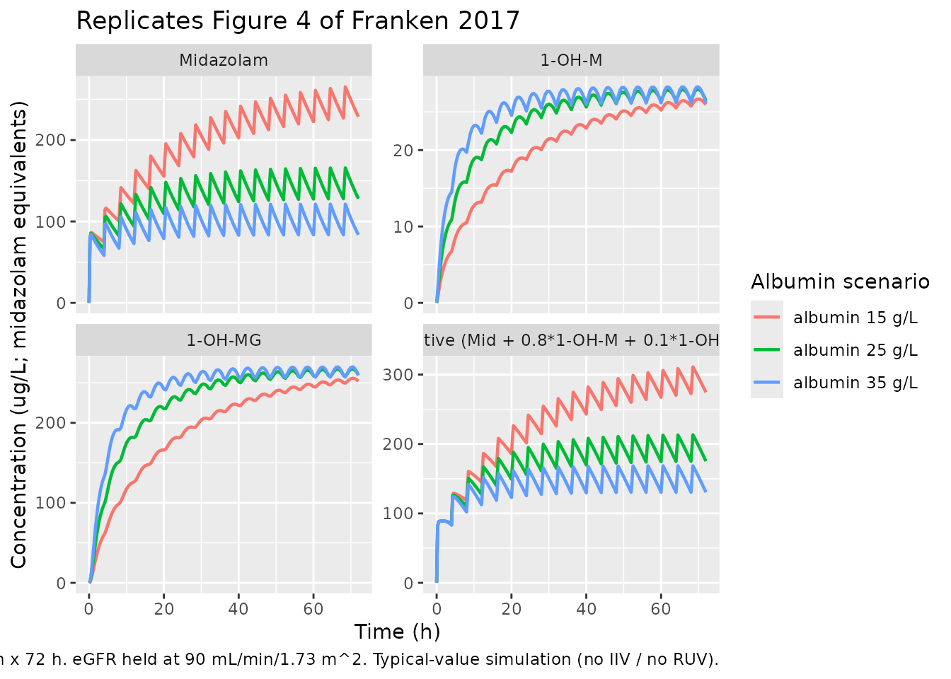
Figure 5: effect of eGFR on midazolam and metabolite concentrations
plot_fig5 <- sim_fig5 |>
  dplyr::mutate(
    Effective = Cc + 0.8 * Cc_1ohm + 0.1 * Cc_1ohmg
  ) |>
  tidyr::pivot_longer(
    cols      = c(Cc, Cc_1ohm, Cc_1ohmg, Effective),
    names_to  = "species",
    values_to = "conc"
  ) |>
  dplyr::mutate(species = factor(
    dplyr::recode(species,
                  "Cc"        = "Midazolam",
                  "Cc_1ohm"   = "1-OH-M",
                  "Cc_1ohmg"  = "1-OH-MG",
                  "Effective" = "Effective (Mid + 0.8*1-OH-M + 0.1*1-OH-MG)"),
    levels = c("Midazolam", "1-OH-M", "1-OH-MG",
               "Effective (Mid + 0.8*1-OH-M + 0.1*1-OH-MG)")
  ))

ggplot(plot_fig5, aes(x = time, y = conc, color = scenario)) +
  geom_line(linewidth = 0.8) +
  facet_wrap(~species, scales = "free_y", ncol = 2) +
  labs(x = "Time (h)",
       y = "Concentration (ug/L; midazolam equivalents)",
       color = "eGFR scenario",
       title = "Replicates Figure 5 of Franken 2017",
       caption = paste(
         "10 mg subcutaneous midazolam loading dose then 5 mg SC every 4 h x 72 h.",
         "Albumin held at 25 g/L.",
         "Typical-value simulation (no IIV / no RUV)."
       ))
Numeric checks against the Discussion / Simulations section
Franken 2017 ‘Simulations’ quotes four numeric anchor results from
the final model. The model file’s ini() reproduces these
closed-form, so the table below also serves as a direct provenance audit
for the two covariate coefficients.
typical_CL <- function(theta_pop, cov, cov_ref, exponent) {
  theta_pop * (cov / cov_ref)^exponent
}

anchor <- tibble::tribble(
  ~quantity,                       ~scenario,                    ~paper,  ~model,
  "Midazolam CL (L/h)",            "ALB = 35 g/L (ref 25, exp 1.08)",
                                                                  12.1,
                                                                  typical_CL(8.42, 35, 25, 1.08),
  "Midazolam CL (L/h)",            "ALB = 25 g/L (reference)",     8.4,
                                                                  typical_CL(8.42, 25, 25, 1.08),
  "Midazolam CL (L/h)",            "ALB = 15 g/L",                 4.8,
                                                                  typical_CL(8.42, 15, 25, 1.08),
  "Midazolam CL (L/h)",            "ALB = 45 g/L (healthy)",       15.3,
                                                                  typical_CL(8.42, 45, 25, 1.08),
  "1-OH-MG CL (L/h)",              "eGFR = 90 (ref 104, exp 0.53)",
                                                                   4.7,
                                                                   typical_CL(5.10, 90, 104, 0.53),
  "1-OH-MG CL (L/h)",              "eGFR = 50",                    3.5,
                                                                   typical_CL(5.10, 50, 104, 0.53),
  "1-OH-MG CL (L/h)",              "eGFR = 30",                    2.7,
                                                                   typical_CL(5.10, 30, 104, 0.53)
) |>
  dplyr::mutate(
    diff_pct = round(100 * (model - paper) / paper, 1)
  )

knitr::kable(
  anchor,
  caption = paste(
    "Typical-value covariate-anchored CL predictions vs Franken 2017",
    "Discussion / Simulations text. Sub-3% differences trace to rounding",
    "of the published coefficients (1.08 and 0.53) and reference values",
    "(median ALB 25 g/L, median eGFR 104 mL/min/1.73 m^2)."
  ),
  align = c("l", "l", "r", "r", "r")
)| quantity | scenario | paper | model | diff_pct |
|---|---|---|---|---|
| Midazolam CL (L/h) | ALB = 35 g/L (ref 25, exp 1.08) | 12.1 | 12.109616 | 0.1 |
| Midazolam CL (L/h) | ALB = 25 g/L (reference) | 8.4 | 8.420000 | 0.2 |
| Midazolam CL (L/h) | ALB = 15 g/L | 4.8 | 4.849706 | 1.0 |
| Midazolam CL (L/h) | ALB = 45 g/L (healthy) | 15.3 | 15.885701 | 3.8 |
| 1-OH-MG CL (L/h) | eGFR = 90 (ref 104, exp 0.53) | 4.7 | 4.723795 | 0.5 |
| 1-OH-MG CL (L/h) | eGFR = 50 | 3.5 | 3.459367 | -1.2 |
| 1-OH-MG CL (L/h) | eGFR = 30 | 2.7 | 2.638863 | -2.3 |
PKNCA validation
Single-dose NCA after the first 10 mg subcutaneous midazolam loading dose (window 0-4 h, before the second dose), computed separately for each analyte and grouped by the eGFR scenarios of Figure 5. This exercises the parent + both metabolites within a single NONMEM-style cohort. The paper itself does not report a baseline NCA table (sparse-sampling design with no IV reference arm), so this section validates that PKNCA runs cleanly on the simulated profiles and surfaces the dose-proportional response in midazolam Cmax with no dependence on eGFR (as expected – eGFR only affects 1-OH-MG CL).
sim_nca_window <- sim_fig5 |> dplyr::filter(time <= 4)

dose_df_fig5 <- events_fig5 |>
  dplyr::filter(evid == 1L, time == 0) |>
  dplyr::select(id, time, amt, scenario)

intervals_sd <- data.frame(
  start     = 0,
  end       = 4,
  cmax      = TRUE,
  tmax      = TRUE,
  auclast   = TRUE,
  half.life = FALSE
)
Midazolam
# Guarantee a time = 0 anchor row per (id, scenario) for PKNCA AUC0-*
add_t0 <- function(df, value_col) {
  df_t0 <- df |>
    dplyr::distinct(id, scenario) |>
    dplyr::mutate(time = 0, !!value_col := 0)
  dplyr::bind_rows(df, df_t0) |>
    dplyr::distinct(id, scenario, time, .keep_all = TRUE) |>
    dplyr::arrange(id, scenario, time)
}

sim_nca_midaz <- sim_nca_window |>
  dplyr::filter(!is.na(Cc)) |>
  dplyr::select(id, time, Cc, scenario) |>
  add_t0("Cc")

conc_obj_midaz <- PKNCA::PKNCAconc(
  sim_nca_midaz, Cc ~ time | scenario + id,
  concu = "ug/L", timeu = "h"
)
dose_obj <- PKNCA::PKNCAdose(
  dose_df_fig5, amt ~ time | scenario + id, doseu = "mg"
)

nca_midaz <- PKNCA::pk.nca(
  PKNCA::PKNCAdata(conc_obj_midaz, dose_obj, intervals = intervals_sd)
)
knitr::kable(as.data.frame(summary(nca_midaz)),
caption = "Midazolam NCA over 4 h after the first 10 mg SC bolus.")| Interval Start | Interval End | scenario | N | AUClast (h*ug/L) | Cmax (ug/L) | Tmax (h) |
|---|---|---|---|---|---|---|
| 0 | 4 | eGFR 10 mL/min | 1 | 295 | 85.3 | 0.500 |
| 0 | 4 | eGFR 30 mL/min | 1 | 295 | 85.3 | 0.500 |
| 0 | 4 | eGFR 60 mL/min | 1 | 295 | 85.3 | 0.500 |
| 0 | 4 | eGFR 90 mL/min | 1 | 295 | 85.3 | 0.500 |
1-OH-M
sim_nca_1ohm <- sim_nca_window |>
  dplyr::filter(!is.na(Cc_1ohm)) |>
  dplyr::select(id, time, Cc_1ohm, scenario) |>
  dplyr::rename(Cc = Cc_1ohm) |>
  add_t0("Cc")

conc_obj_1ohm <- PKNCA::PKNCAconc(
  sim_nca_1ohm, Cc ~ time | scenario + id,
  concu = "ug/L", timeu = "h"
)
nca_1ohm <- PKNCA::pk.nca(
  PKNCA::PKNCAdata(conc_obj_1ohm, dose_obj, intervals = intervals_sd)
)
knitr::kable(as.data.frame(summary(nca_1ohm)),
caption = "1-OH-M NCA over 4 h after the first 10 mg SC midazolam bolus.")| Interval Start | Interval End | scenario | N | AUClast (h*ug/L) | Cmax (ug/L) | Tmax (h) |
|---|---|---|---|---|---|---|
| 0 | 4 | eGFR 10 mL/min | 1 | 28.5 | 10.9 | 4.00 |
| 0 | 4 | eGFR 30 mL/min | 1 | 28.5 | 10.9 | 4.00 |
| 0 | 4 | eGFR 60 mL/min | 1 | 28.5 | 10.9 | 4.00 |
| 0 | 4 | eGFR 90 mL/min | 1 | 28.5 | 10.9 | 4.00 |
1-OH-MG
sim_nca_1ohmg <- sim_nca_window |>
  dplyr::filter(!is.na(Cc_1ohmg)) |>
  dplyr::select(id, time, Cc_1ohmg, scenario) |>
  dplyr::rename(Cc = Cc_1ohmg) |>
  add_t0("Cc")

conc_obj_1ohmg <- PKNCA::PKNCAconc(
  sim_nca_1ohmg, Cc ~ time | scenario + id,
  concu = "ug/L", timeu = "h"
)
nca_1ohmg <- PKNCA::pk.nca(
  PKNCA::PKNCAdata(conc_obj_1ohmg, dose_obj, intervals = intervals_sd)
)
knitr::kable(as.data.frame(summary(nca_1ohmg)),
caption = "1-OH-MG NCA over 4 h after the first 10 mg SC midazolam bolus.")| Interval Start | Interval End | scenario | N | AUClast (h*ug/L) | Cmax (ug/L) | Tmax (h) |
|---|---|---|---|---|---|---|
| 0 | 4 | eGFR 10 mL/min | 1 | 412 | 231 | 4.00 |
| 0 | 4 | eGFR 30 mL/min | 1 | 312 | 159 | 4.00 |
| 0 | 4 | eGFR 60 mL/min | 1 | 247 | 118 | 4.00 |
| 0 | 4 | eGFR 90 mL/min | 1 | 212 | 97.9 | 4.00 |
Assumptions and deviations
-
Residual-error interpretation. Franken 2017 Methods
‘Base model development’ reports residual variability as “additive
residual error on logarithmic transformed concentrations” (LTBS), with
Table 2 Final values reported as CV percentages (26.8% / 42.3% / 46.4%
for midazolam / 1-OH-M / 1-OH-MG). The packaged model converts each CV
via the canonical log-normal identity
omega^2 = log(1 + CV^2)and passes the square root to rxode2’slnorm()residual model. The Franken 2015 morphine paper from the same group reports residual variability as raw NONMEM$SIGMAvariance values (no percent sign); the difference in reporting style is paper-specific. Both interpretations of the midazolam Table 2 values (CV% -> log-normal conversion versus log-scale SD directly) give numerically indistinguishable predictions for CV <= 0.5. -
Cross-output residual correlation not encoded.
Franken 2017 Methods ‘Base model development’ notes that “since the
parent and metabolite concentrations were measured in the same samples
using a single assay, a correlation between the residual errors was
incorporated in the model.” The paper does not report the correlation
magnitude in Table 2, and rxode2 / nlmixr2 do not support cross-output
residual correlations directly via the
Cc ~ lnorm(expSd)interface. The packaged model treats the three residuals as independent, which slightly underestimates the joint shrinkage of simulated parent-vs-metabolite trajectories at any single time point. Marginal univariate VPCs and per-output NCA summaries are unaffected. -
1-OH-M volume of distribution. The packaged model
sets
vc_1ohm = vc(a structural equality, not a separately estimated parameter), matching Methods ‘Base model development’: “The volume of distribution (V) of 1-OH-M was assumed to be equal to the volume of distribution of midazolam.” - Apparent vs absolute clearance. Per Discussion: “the 4-OH-M metabolite was not included in the model and the true fraction metabolized is unknown, the clearance and distribution volumes of the other metabolites are apparent values.” The packaged model uses the published apparent values directly without attempting to back out fractions; downstream users who want absolute clearance should rescale by their own assumed fraction-metabolised.
-
Absorption rate constants fixed from literature.
Methods ‘Structural model’: “the absorption constants (Ka) could not be
estimated. They were therefore derived from literature (5.5 h^-1 for
oral administration, 10 h^-1 for subcutaneous injection).” Wrapped in
fixed()in the model file; both values are structural assumptions, not estimated. -
SC bioavailability assumed 1. Methods ‘Base model
development’: “Bioavailability of subcutaneous midazolam was assumed to
be 100%.” The packaged model leaves the SC depot’s bioavailability at
the rxode2 default 1 (no
f(depot2) <- ...assignment) and estimates oral F vialfdepot. -
F-vs-CL correlation fixed to unity. Methods ‘Base
model development’: “The correlation between IIV of midazolam clearance
and F of oral midazolam was high (0.93) and therefore fixed to unity.”
Encoded as a 2x2 OMEGA block with off-diagonal
sqrt(var_F * var_CL), which is mathematically equivalent to the published shared-eta-with-scaling-theta NONMEM construct. - eGFR formula. The packaged model uses the standard four-variable MDRD eGFR (paper’s “eGFR-a”, Methods Eq. 4), which is the equation retained in the Final model. The original six-variable MDRD formula (“eGFR-b”, Eq. 5) was tested but not retained because the difference in fit was minimal.
-
Time-to-death (TTD) not retained. TTD was tested as
a covariate on midazolam CL (delta-OFV = -4.69), midazolam V (delta-OFV
= -6.50), and 1-OH-MG CL (delta-OFV = -15.25) per Table 3, but did not
survive backward elimination at p < 0.001. The packaged model omits
TTD accordingly. The Franken 2015 companion morphine model
(
modellib("Franken_2015_morphine")) retains TTD on parent CL because it did clear the morphine paper’s stricter selection process. - Bootstrap-derived 95% confidence intervals not surfaced. Table 2 reports bootstrap (200-run) 95% CI bounds for every estimate. The model file carries only the Final-model point estimates; the bootstrap CIs are documented in the paper’s Table 2 and the in-file comments reference them implicitly via the RSE column.
- NPDE not reproduced. The paper validated the final model via NPDE (global adjusted p = 0.75 / 0.20 / 0.41 for the three analytes), not VPC, because of the variable dosing-regimen design that precludes a standard VPC. The packaged vignette replicates the typical-value Figure 4 / Figure 5 simulations (the only quantitative figures the paper presents) rather than re-running NPDE.