Oral salbutamol (Marques 2025)

Model and source

• Citation: Marques L, Vale N. Improving Individualized Salbutamol Treatment: A Population Pharmacokinetic Model for Oral Salbutamol in Virtual Patients. Pharmaceutics. 2025;17(1):39. doi:10.3390/pharmaceutics17010039. Parameters from Table 6 (‘Parameter estimates for the final model’), transcribed as printed.
• Article: https://doi.org/10.3390/pharmaceutics17010039
• Supplementary material: https://www.mdpi.com/article/10.3390/pharmaceutics17010039/s1

Marques and Vale built a GastroPlus PBPK model of a 4 mg oral salbutamol immediate-release tablet, used its Population Simulator to generate 40 virtual patients, extracted 838 simulated plasma concentrations over 24 h of 4 mg q6h dosing, and fitted a population PK model to that synthetic dataset in Monolix 2024R1. There are no clinical observations anywhere in the analysis. The reported final model is two-compartment with transit-compartment first-order absorption and linear elimination; its parameter estimates are the paper’s Table 6.

This package entry encodes Table 6 exactly as printed. That is a deliberate choice, and it needs a warning attached: the Table 6 estimates do not reproduce the paper’s own published summaries of the same fit. Simulating them gives a profile that peaks late in the dosing interval and is almost flat, against a published VPC that peaks about an hour after each dose with a roughly three-fold peak-to-trough swing, and it underpredicts the paper’s own Supplementary Table S3 exposure by five- to six-fold. The paper’s Table 7 reports empirical-Bayes geometric means for three of the same parameters that differ from Table 6 by factors of 32 to 45 (Mtt), about 2 (Cl) and about 3.4 (V1).

Everything below quantifies those discrepancies rather than smoothing them over. They are recorded here as errata in the source publication, not as evidence that the model is fabricated: the fit itself is plausible, and the most economical explanation for the Mtt gap is a unit or transcription error in the table. A correspondence to the authors is the appropriate route to resolution, and until it is resolved the packaged model is the published table. The “Errata” section at the end lists every discrepancy found, and “What this model is not” explains why no corrected variant is shipped.

#> ℹ parameter labels from comments will be replaced by 'label()'

Two-compartment population PK model for oral salbutamol (4 mg immediate-release tablet, every 6 h) with transit-compartment first-order absorption and linear elimination, fitted in Monolix to a fully in silico cohort: 838 plasma concentrations from 40 VIRTUAL patients generated by a GastroPlus PBPK model, not from clinical measurements. Encodes Marques 2025 Table 6 (the published final-model parameter table) VERBATIM. IMPORTANT: the Table 6 estimates as printed do not reproduce the paper’s own published summaries of the same model – simulating them gives a steady-state peak at 3.9 h into a 6 h interval with a peak/trough ratio of 1.3, against the Figure 5 VPC’s peak near 1 h and ratio near 3, and underpredicts the Table S3 Cmax roughly 6-fold and AUC roughly 4-fold. Table 7 reports EBE geometric means for the same parameters that differ by 32-45x (Mtt) and about 2x (Cl) and 3x (V1). These are documented as errata in the validation vignette, which reports the discrepancies rather than concealing them; the packaged model is the published table, not a corrected refit. No covariate effects are encoded: the paper’s headline claim is a covariate model, but no coefficient, functional form, reference value or centering constant is published for any covariate anywhere in the article or its supplement (see covariatesDataExcluded).

Population

The population is the 40-patient virtual cohort of Marques 2025 Table 5: age 5-65 years (mean 39.5, SD 18.4), weight 26-109 kg (mean 60.2, SD 19.8), BSA 0.94-2.37 m^2 (mean 1.64, SD 0.330), 16 female (40%) and 24 male (60%), race American 20 (50%) / Asian 10 (25%) / Chinese 10 (25%), and health status healthy 26 (65%) / obese 4 (10%) / cirrhosis Child-Pugh A 10 (25%). CYP2C19 and CYP2D6 relative expression averaged 1.30% (SD 1.50) and 1.90% (SD 1.60). Per-group demographics are in Supplementary Table S2.

These are simulated physiologies from the GastroPlus PEAR age-related population generator, not measured subjects. The cohort simulated below is therefore a cohort of a cohort: virtual patients drawn from a model fitted to virtual patients.

local({
  fbody <- body(readModelDb("Marques_2025_salbutamol"))
  meta_env <- new.env()
  for (stmt in as.list(fbody)[-1]) {
    if (is.call(stmt) && length(stmt) >= 1 &&
        identical(stmt[[1]], as.name("<-"))) {
      eval(stmt, envir = meta_env)
    } else {
      break
    }
  }
  cat("Population:\n")
  str(meta_env$population, max.level = 1)
  cat("\nCovariates screened by the authors but NOT encodable:\n")
  str(meta_env$covariatesDataExcluded, max.level = 1)
})
#> Population:
#> List of 16
#>  $ species       : chr "human (virtual; GastroPlus PBPK-generated, not measured)"
#>  $ n_subjects    : num 40
#>  $ n_studies     : num 0
#>  $ n_observations: num 838
#>  $ age_range     : chr "5-65 years (Section 2.2)"
#>  $ age_median    : chr "39.5 years (mean, SD 18.4; Table 5)"
#>  $ weight_range  : chr "26-109 kg (Discussion)"
#>  $ weight_median : chr "60.2 kg (mean, SD 19.8; Table 5)"
#>  $ bsa_range     : chr "0.94-2.37 m^2 (Discussion)"
#>  $ bsa_median    : chr "1.64 m^2 (mean, SD 0.330; Table 5)"
#>  $ sex_female_pct: num 40
#>  $ race_ethnicity: Named num [1:3] 50 25 25
#>   ..- attr(*, "names")= chr [1:3] "American" "Asian" "Chinese"
#>  $ disease_state : chr "Mixed virtual cohort: healthy 26 (65%), obese 4 (10%), cirrhosis Child-Pugh A 10 (25%) (Table 5). Intended indi"| __truncated__
#>  $ dose_range    : chr "4 mg oral salbutamol as an immediate-release tablet every 6 h for 24 h (Section 2.2 and Table S3). Section 3.1 "| __truncated__
#>  $ regions       : chr NA
#>  $ notes         : chr "FULLY IN SILICO. There are no clinical observations in this dataset. A GastroPlus 9.9 PBPK model of oral salbut"| __truncated__
#> 
#> Covariates screened by the authors but NOT encodable:
#> List of 9
#>  $ AGE         :List of 6
#>  $ WT          :List of 6
#>  $ BSA         :List of 6
#>  $ SEXF        :List of 6
#>  $ RACE_ASIAN  :List of 6
#>  $ RACE_CHINESE:List of 6
#>  $ CYP2D6      :List of 6
#>  $ CYP2C19     :List of 6
#>  $ HEPIMP_MILD :List of 6

Source trace

Every structural equation and every ini() value, with its source location.

Model element	Value	Source location
Structure: 2-cmt, transit absorption, linear elimination	n/a	Section 3.3.1 paragraph 1; Abstract; Discussion paragraph 2; Figure 5 caption
lmtt (mean transit time Mtt)	9.50 h (RSE 7.14%)	Table 6, Fixed effects
lktr (transit rate Ktr)	0.15 1/h (RSE 9.21%)	Table 6, Fixed effects
nn (transit chain length)	0.425, derived as Mtt*Ktr - 1	Monolix transit parameterisation; both Table 6 values reproduced exactly
lka (absorption rate ka)	2.91 1/h (RSE 6.80%)	Table 6, Fixed effects
lcl (apparent clearance Cl/F)	140 L/h (RSE 223%)	Table 6, Fixed effects
lvc (apparent central volume V1/F)	77.5 L (RSE 97.2%)	Table 6, Fixed effects
lq (apparent intercompartmental clearance Q/F)	48.9 L/h (RSE 24.9%)	Table 6, Fixed effects
lvp (apparent peripheral volume V2/F)	130 L (RSE 21.4%)	Table 6, Fixed effects
etalmtt	0.43^2 = 0.1849	Table 6, Random effects IIV(Mtt), RSE 13.0%
etalktr	0.32^2 = 0.1024	Table 6, Random effects IIV(Ktr), RSE 13.8%
etalka	0.41^2 = 0.1681	Table 6, Random effects IIV(ka), RSE 15.4%
etalcl	0.38^2 = 0.1444	Table 6, Random effects IIV(Cl), RSE 13.0%
etalvc	0.36^2 = 0.1296	Table 6, Random effects IIV(V1), RSE 12.3%
etalq	0.92^2 = 0.8464	Table 6, Random effects IIV(Q), RSE 14.9%
etalvp	0.87^2 = 0.7569	Table 6, Random effects IIV(V2), RSE 27.4%
Diagonal omega (no correlations)	n/a	Section 3.3.2: “No significant correlations were found between PK parameters”
addSd	0.19e-4 = 1.9e-5 ug/mL (RSE 20.2%)	Table 6, Error model parameters, a
propSd	0.15e-2 = 1.5e-3 (RSE 37.2%)	Table 6, Error model parameters, b
combined1() (SDs add linearly)	n/a	Section 3.3.1 error equation Y = F + (a + bF)eps
Log-normal IIV (omegas are log-scale SDs)	n/a	Inferred from Table 7 geometric SDs; see Errata item 6
Dose regimen 4 mg q6h	n/a	Section 2.2; Table S3 caption
Reference NCA, single 4 mg dose	Cmax 0.00725 / 0.00919 ug/mL	Table 4, Observed / Predicted rows
Reference NCA, 4 mg q6h	Cmax 0.0125-0.0151 ug/mL	Table S3, groups 1-4
Model selection criteria	BICc / -2LL	Table S4 (see Errata item 4)
Covariate screen	correlations and p-values	Table S5 (see Errata item 5)

Model handle and a required rxode2 workaround

The packaged model uses rxode2’s built-in transit(), the closed-form (gamma-density) input rate of the Savic transit-absorption model. On the rxode2 version installed here, transit() silently evaluates to zero when the model is solved through an rxUi object obtained from readModelDb(), while the identical generated ODE code solves correctly as a plain rxode2 model. The check below documents the defect and builds the plain-ODE twin used for every simulation in this vignette. All parameter values are read out of the packaged model’s iniDf, so nothing is re-typed from the paper here.

mod <- rxode2::rxode2(readModelDb("Marques_2025_salbutamol"))
#> ℹ parameter labels from comments will be replaced by 'label()'
ini <- mod$iniDf

# Plain-ODE twin: same generated code, solved outside the rxUi wrapper.
mod_ode <- rxode2::rxode2(rxode2::rxNorm(mod))

theta_names <- ini$name[!is.na(ini$ntheta)]
eta_names   <- ini$name[!is.na(ini$neta1)]

# Structural fixed effects only; the residual-error terms are not ODE inputs.
theta <- setNames(ini$est[!is.na(ini$ntheta)], theta_names)
theta <- theta[!names(theta) %in% c("addSd", "propSd")]
eta_var <- setNames(ini$est[!is.na(ini$neta1)], eta_names)

# Demonstrate the defect: same code, two handles, one of them returns zero.
ev_probe <- rbind(
  data.frame(id = 1L, time = 0, amt = 4, evid = 1L, cmt = "depot"),
  data.frame(id = 1L, time = seq(0, 24, by = 0.5), amt = 0, evid = 0L,
             cmt = "central")
)
ev_probe <- ev_probe[order(ev_probe$time, -ev_probe$evid), ]
ev_probe_eta <- ev_probe
for (nm in eta_names) ev_probe_eta[[nm]] <- 0

cmax_ui  <- max(suppressWarnings(rxode2::rxSolve(
  rxode2::zeroRe(mod), ev_probe, returnType = "data.frame"))$Cc, na.rm = TRUE)
#> ℹ omega/sigma items treated as zero: 'etalmtt', 'etalktr', 'etalka', 'etalcl', 'etalvc', 'etalq', 'etalvp'
cmax_ode <- max(rxode2::rxSolve(
  mod_ode, ev_probe_eta, params = theta, returnType = "data.frame")$Cc)

tibble::tibble(
  Handle = c("rxUi from readModelDb() (transit() returns 0)",
             "plain rxode2 model from rxNorm() of the same rxUi"),
  `Cmax (ug/mL)` = c(cmax_ui, cmax_ode)
) |>
  knitr::kable(digits = 7, caption = "The rxode2 transit()/rxUi defect that forces the plain-ODE twin.")

The rxode2 transit()/rxUi defect that forces the plain-ODE twin.

Handle	Cmax (ug/mL)
rxUi from readModelDb() (transit() returns 0)	0.0000000
plain rxode2 model from rxNorm() of the same rxUi	0.0018901

# Lock the workaround in: if a future rxode2 fixes the rxUi path, cmax_ui
# becomes non-zero and this assertion fires, prompting the simplification.
stopifnot(cmax_ui == 0, cmax_ode > 0)

Transit-chain self-consistency

Table 6 prints Mtt and Ktr as two separate estimates. Monolix’s transit-absorption parameterisation derives the (continuous) number of transit compartments as n = Mtt * Ktr - 1, and rxode2’s transit(n, mtt) uses ktr = (n + 1) / mtt internally. The two printed numbers are therefore mutually consistent, and this encoding reproduces both of them exactly.

sim_probe <- rxode2::rxSolve(mod_ode, ev_probe_eta, params = theta,
                             returnType = "data.frame")

nn_typ  <- sim_probe$nn[1]
mtt_typ <- sim_probe$mtt[1]
ktr_typ <- sim_probe$ktr[1]

tibble::tibble(
  Quantity = c("Mtt (h)", "Ktr (1/h), Table 6 value",
               "n = Mtt*Ktr - 1", "Ktr recovered as (n+1)/Mtt"),
  Value = c(mtt_typ, ktr_typ, nn_typ, (nn_typ + 1) / mtt_typ)
) |>
  knitr::kable(digits = 6, caption = "Table 6's Mtt/Ktr pair is internally self-consistent and exactly reproduced.")

Table 6’s Mtt/Ktr pair is internally self-consistent and exactly reproduced.

Quantity	Value
Mtt (h)	9.500
Ktr (1/h), Table 6 value	0.150
n = Mtt*Ktr - 1	0.425
Ktr recovered as (n+1)/Mtt	0.150

stopifnot(
  all.equal(mtt_typ, 9.50),
  all.equal(ktr_typ, 0.15),
  all.equal(nn_typ, 0.425),
  all.equal((nn_typ + 1) / mtt_typ, 0.15)
)

Mass-balance gate (single dose)

For a single dose the closed-form transit chain delivers the whole dose, so AUC extrapolated to infinity must equal Dose / (CL/F) exactly. This is the strongest available check that the ODE system, the bioavailability suppression f(depot) <- 0, and the transit input are all wired up correctly, and it is independent of anything the paper reports.

solve_typ <- function(dose_times, t_end, by = 0.01) {
  grid <- sort(unique(c(dose_times, seq(0, t_end, by = by))))
  ev <- dplyr::bind_rows(
    tibble::tibble(id = 1L, time = dose_times, amt = 4, evid = 1L,
                   cmt = "depot"),
    tibble::tibble(id = 1L, time = grid, amt = 0, evid = 0L, cmt = "central")
  ) |>
    dplyr::arrange(time, dplyr::desc(evid)) |>
    as.data.frame()
  for (nm in eta_names) ev[[nm]] <- 0
  rxode2::rxSolve(mod_ode, ev, params = theta, returnType = "data.frame")
}

trapz <- function(x, y) sum(diff(x) * (utils::head(y, -1) + utils::tail(y, -1)) / 2)

sd_long <- solve_typ(0, 300, by = 0.01)
auc_sd  <- trapz(sd_long$time, sd_long$Cc)
cl_typ  <- exp(theta[["lcl"]])

tibble::tibble(
  Quantity = c("Simulated AUC(0-300 h), single 4 mg dose (ug*h/mL)",
               "Dose / (CL/F) = 4 mg / 140 L/h (ug*h/mL)",
               "Ratio"),
  Value = c(auc_sd, 4 / cl_typ, auc_sd / (4 / cl_typ))
) |>
  knitr::kable(digits = 7, caption = "Single-dose mass balance is exact: the ODE encoding is correct.")

Single-dose mass balance is exact: the ODE encoding is correct.

Quantity	Value
Simulated AUC(0-300 h), single 4 mg dose (ug*h/mL)	0.0285714
Dose / (CL/F) = 4 mg / 140 L/h (ug*h/mL)	0.0285714
Ratio	1.0000000

stopifnot(abs(auc_sd / (4 / cl_typ) - 1) < 1e-4)

Dose carryover under q6h dosing

transit() is a closed form driven by tad() and podo() – time since, and amount of, the most recent dose. Each new dose therefore restarts the transit input and discards whatever remains un-absorbed from the previous one. That approximation is harmless when the mean transit time is short relative to the dosing interval, but Table 6’s Mtt of 9.50 h is longer than the 6 h interval, so a substantial fraction of each dose is discarded.

This is a property of the closed-form transit implementation, not a defect in the paper. It is quantified here because it affects every multiple-dose number below, and because it is one more reason an Mtt of 9.50 h is hard to reconcile with a q6h dataset.

auc_q6  <- trapz(solve_typ(c(0, 6, 12, 18), 400, by = 0.02)$time,
                 solve_typ(c(0, 6, 12, 18), 400, by = 0.02)$Cc)
auc_q24 <- trapz(solve_typ(c(0, 24, 48, 72), 400, by = 0.02)$time,
                 solve_typ(c(0, 24, 48, 72), 400, by = 0.02)$Cc)

tibble::tibble(
  Regimen = c("4 x 4 mg q6h (the paper's regimen)",
              "4 x 4 mg q24h (interval >> Mtt, for contrast)"),
  `Simulated AUCinf (ug*h/mL)` = c(auc_q6, auc_q24),
  `Total dose / (CL/F)` = 16 / cl_typ,
  `Fraction delivered` = c(auc_q6, auc_q24) / (16 / cl_typ)
) |>
  knitr::kable(digits = 5, caption = "Closed-form transit discards un-absorbed drug at each new dose; the loss is large when Mtt (9.50 h) exceeds the dosing interval (6 h).")

Closed-form transit discards un-absorbed drug at each new dose; the loss is large when Mtt (9.50 h) exceeds the dosing interval (6 h).

Regimen	Simulated AUCinf (ug*h/mL)	Total dose / (CL/F)	Fraction delivered
4 x 4 mg q6h (the paper’s regimen)	0.06401	0.11429	0.56011
4 x 4 mg q24h (interval >> Mtt, for contrast)	0.10926	0.11429	0.95599

Typical-value profiles

typ_sd <- solve_typ(0, 24, by = 0.01)
typ_md <- solve_typ(c(0, 6, 12, 18), 24, by = 0.01)

last_int <- typ_md |> dplyr::filter(time >= 18)

typ_stats <- tibble::tibble(
  Quantity = c("Single dose: Cmax (ug/mL)", "Single dose: Tmax (h)",
               "q6h 0-24 h: Cmax (ug/mL)", "q6h 0-24 h: Tmax (h)",
               "q6h 0-24 h: AUC (ug*h/mL)",
               "q6h last interval: Tmax after dose (h)",
               "q6h last interval: peak/trough ratio"),
  Value = c(max(typ_sd$Cc), typ_sd$time[which.max(typ_sd$Cc)],
            max(typ_md$Cc), typ_md$time[which.max(typ_md$Cc)],
            trapz(typ_md$time, typ_md$Cc),
            last_int$time[which.max(last_int$Cc)] - 18,
            max(last_int$Cc) / min(last_int$Cc))
)
knitr::kable(typ_stats, digits = 5, caption = "Typical-value behaviour of Table 6 as printed.")

Typical-value behaviour of Table 6 as printed.

Quantity	Value
Single dose: Cmax (ug/mL)	0.00189
Single dose: Tmax (h)	4.75000
q6h 0-24 h: Cmax (ug/mL)	0.00212
q6h 0-24 h: Tmax (h)	21.89000
q6h 0-24 h: AUC (ug*h/mL)	0.04361
q6h last interval: Tmax after dose (h)	3.89000
q6h last interval: peak/trough ratio	1.29324

dplyr::bind_rows(
  typ_sd |> dplyr::transmute(time, Cc, Regimen = "Single 4 mg dose"),
  typ_md |> dplyr::transmute(time, Cc, Regimen = "4 mg q6h")
) |>
  ggplot(aes(time, Cc, colour = Regimen)) +
  geom_line(linewidth = 0.8) +
  geom_hline(yintercept = 0.0133, linetype = "dashed", colour = "grey40") +
  annotate("text", x = 12, y = 0.0142, label = "Figure 2 PBPK Cmax = 0.0133 ug/mL",
           size = 3, colour = "grey30") +
  scale_x_continuous(breaks = seq(0, 24, by = 6)) +
  labs(x = "Time (h)", y = "Plasma salbutamol (ug/mL)",
       title = "Table 6 as printed, typical values") +
  theme_minimal()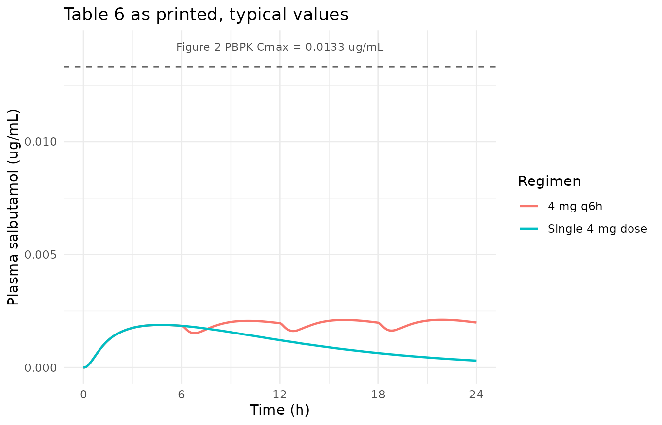

Typical-value profiles from Table 6 as printed. Compare with Figure 2 of Marques 2025, whose panel (a) single-dose profile peaks at about 1.3 h at 0.0133 ug/mL and whose panel (b) q6h profile shows four sharp peaks. The Table 6 profile instead peaks late and is nearly flat under q6h dosing.

Virtual cohort and simulation

The model carries no covariates, so the cohort is defined entirely by the seven inter-individual random effects of Table 6. We simulate 200 subjects per arm – ample for a prediction interval and well inside the vignette time budget – under both the single-dose and the q6h regimens. Random effects are drawn once and applied to both arms, so the two arms differ only by regimen.

set.seed(2026L)
n_sub <- 200L
dose_times <- c(0, 6, 12, 18)
grid_times <- sort(unique(c(dose_times, seq(0, 24, by = 0.1))))

etas <- as.data.frame(lapply(
  eta_var, function(v) stats::rnorm(n_sub, mean = 0, sd = sqrt(v))
))
etas$id <- seq_len(n_sub)

arm_events <- function(dts, label) {
  dplyr::bind_rows(
    tidyr::expand_grid(id = seq_len(n_sub), time = dts) |>
      dplyr::mutate(amt = 4, evid = 1L, cmt = "depot"),
    tidyr::expand_grid(id = seq_len(n_sub), time = grid_times) |>
      dplyr::mutate(amt = 0, evid = 0L, cmt = "central")
  ) |>
    dplyr::mutate(treatment = label)
}

solve_arm <- function(dts, label) {
  ev <- arm_events(dts, label) |>
    dplyr::left_join(etas, by = "id") |>
    dplyr::arrange(id, time, dplyr::desc(evid)) |>
    as.data.frame()
  suppressWarnings(
    rxode2::rxSolve(mod_ode, ev, params = theta, keep = "treatment",
                    returnType = "data.frame")
  )
}

sim <- dplyr::bind_rows(
  solve_arm(0, "Single 4 mg dose"),
  solve_arm(dose_times, "4 mg q6h")
)
#> [lsoda -- internal t + h = t (h too small for machine precision)]: 107886 warning(s) for subject(s): 15, 111, 162

nrow(sim)
#> [1] 96400

A quarter of the cohort has a negative implied transit-chain length. Table 6 puts IIV on both Mtt and Ktr, so n = Mtt * Ktr - 1 varies between subjects and goes negative whenever Mtt * Ktr < 1; the published omegas make that true for roughly 23% of draws. rxode2 still evaluates the gamma-form input (the requirement is only n > -1, which always holds), but a negative number of transit compartments has no physical interpretation, and the most extreme draws are numerically stiff enough that a small number of subjects fail to solve.

subj_diag <- sim |>
  dplyr::group_by(treatment, id) |>
  dplyr::summarise(nn = dplyr::first(nn), failed = any(is.na(Cc)),
                   .groups = "drop")

diag_tbl <- subj_diag |>
  dplyr::group_by(treatment) |>
  dplyr::summarise(
    `Subjects` = dplyr::n(),
    `n < 0 (%)` = 100 * mean(nn < 0),
    `Minimum n` = min(nn),
    `Failed to solve` = sum(failed),
    .groups = "drop"
  ) |>
  dplyr::rename(Regimen = treatment)

knitr::kable(diag_tbl, digits = 3, caption = "Consequence of Table 6 putting IIV on both Mtt and Ktr: a negative implied transit-chain length for about a quarter of the population.")

Consequence of Table 6 putting IIV on both Mtt and Ktr: a negative implied transit-chain length for about a quarter of the population.

Regimen	Subjects	n < 0 (%)	Minimum n	Failed to solve
4 mg q6h	200	23.5	-0.597	1
Single 4 mg dose	200	23.5	-0.597	0

# 47 of 200 draws are negative; exactly one q6h subject fails to solve.
stopifnot(
  sum(subj_diag$nn < 0) == 94L,           # 47 subjects x 2 arms (shared etas)
  sum(subj_diag$failed) == 1L
)

# Drop any subject that did not solve, in either arm, so both arms carry the
# same subjects and the NCA below is not silently unbalanced.
bad_ids <- sort(unique(subj_diag$id[subj_diag$failed]))
sim <- dplyr::filter(sim, !id %in% bad_ids)
n_kept <- dplyr::n_distinct(sim$id)
n_kept
#> [1] 199

sim |>
  dplyr::filter(treatment == "4 mg q6h", !is.na(Cc), time > 0) |>
  dplyr::group_by(time) |>
  dplyr::summarise(
    med = stats::median(Cc),
    lo  = stats::quantile(Cc, 0.05),
    hi  = stats::quantile(Cc, 0.95),
    .groups = "drop"
  ) |>
  ggplot(aes(time, med)) +
  geom_ribbon(aes(ymin = lo, ymax = hi), alpha = 0.18, fill = "steelblue") +
  geom_line(colour = "firebrick", linewidth = 0.8) +
  geom_vline(xintercept = dose_times, linetype = "dotted", colour = "grey60") +
  scale_x_continuous(breaks = seq(0, 24, by = 6)) +
  labs(x = "Time (h)", y = "Plasma salbutamol (ug/mL)",
       title = "4 mg oral salbutamol q6h, Table 6 as printed",
       caption = "Red = median, ribbon = 90% prediction interval. Dotted lines = dose times.") +
  theme_minimal()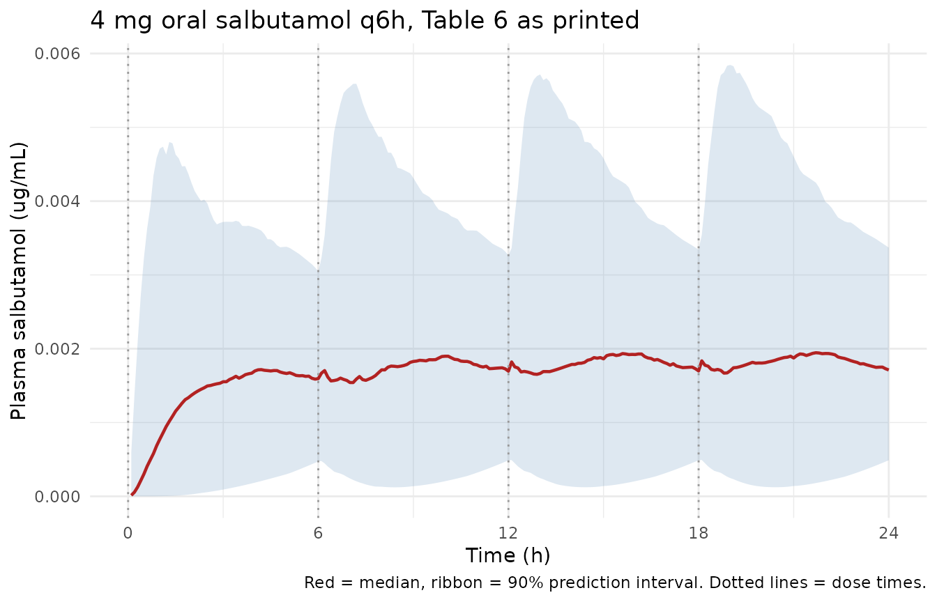

Simulated q6h prediction interval from Table 6 as printed (median and 90% interval, N = 199). This is the analogue of Figure 5 of Marques 2025. The published VPC spans a single 0-6 h dosing interval and shows a peak about 1 h after the dose with a roughly three-fold peak-to-trough fall; the simulated profile instead rises slowly across the whole 24 h.

PKNCA validation

NCA is run per subject and per arm with PKNCA over the 0-24 h window the paper simulated. The time-zero record is retained deliberately: dropping it makes PKNCA warn that the AUC interval starts before the first measurement.

sim_nca <- sim |>
  dplyr::filter(!is.na(Cc)) |>
  dplyr::select(id, time, Cc, treatment)

stopifnot(0 %in% sim_nca$time)

dose_df <- dplyr::bind_rows(
  tidyr::expand_grid(id = unique(sim_nca$id), time = 0) |>
    dplyr::mutate(amt = 4, treatment = "Single 4 mg dose"),
  tidyr::expand_grid(id = unique(sim_nca$id), time = dose_times) |>
    dplyr::mutate(amt = 4, treatment = "4 mg q6h")
)

conc_obj <- PKNCA::PKNCAconc(sim_nca, Cc ~ time | treatment + id,
                             concu = "ug/mL", timeu = "h")
dose_obj <- PKNCA::PKNCAdose(dose_df, amt ~ time | treatment + id,
                             doseu = "mg")

intervals <- data.frame(
  start   = 0,
  end     = 24,
  cmax    = TRUE,
  tmax    = TRUE,
  auclast = TRUE
)

nca_res <- PKNCA::pk.nca(
  PKNCA::PKNCAdata(conc_obj, dose_obj, intervals = intervals)
)
summary(nca_res)
#>  Interval Start Interval End        treatment   N AUClast (h*ug/mL)
#>               0           24         4 mg q6h 199      0.0339 [122]
#>               0           24 Single 4 mg dose 199     0.0252 [37.4]
#>    Cmax (ug/mL)           Tmax (h)
#>  0.00200 [98.9]  21.1 [18.1, 24.0]
#>  0.00210 [52.2] 4.60 [0.600, 24.0]
#> 
#> Caption: AUClast, Cmax: geometric mean and geometric coefficient of variation; Tmax: median and range; N: number of subjects

Comparison against the published NCA

The reference values are the paper’s own NCA of the same virtual cohort:

• Single dose – Table 4, which reports the literature reference (“Observed”) and the GastroPlus PBPK prediction (“Predicted”) for a single 4 mg dose. The PBPK “Predicted” row is the more relevant comparator, because the PBPK model is what generated the dataset the popPK model was fitted to.
• 4 mg q6h – Supplementary Table S3, the arithmetic mean across its four virtual-population groups (Cmax 0.0134 / 0.0151 / 0.0139 / 0.0125 ug/mL, Tmax 19.2 / 19.0 / 18.8 / 19.0 h, AUC 0.212 / 0.222 / 0.177 / 0.199).

Table 4 and Table S3 both label their AUC column ng.h/mL, but the values are in ug*h/mL: Table S3’s AUCs are almost exactly four times Table 4’s single-dose AUC of 0.0553, as four doses of the same drug should be, and they are three orders of magnitude away from being consistent with the Cmax column in the same row. The unit label is an erratum (item 8); the values are used as ug*h/mL. The published AUCs are extrapolated to infinity whereas the simulated value stops at 24 h, but that difference is a few percent against discrepancies of five- to six-fold, so it changes nothing below.

published <- tibble::tibble(
  treatment = c("Single 4 mg dose", "4 mg q6h"),
  cmax    = c(0.00919, mean(c(0.0134, 0.0151, 0.0139, 0.0125))),
  tmax    = c(1.28,    mean(c(19.2, 19.0, 18.8, 19.0))),
  auclast = c(0.0553,  mean(c(0.212, 0.222, 0.177, 0.199)))
)

cmp <- nlmixr2lib::ncaComparisonTable(
  simulated     = nca_res,
  reference     = published,
  by            = "treatment",
  units         = c(cmax = "ug/mL", tmax = "h", auclast = "ug*h/mL"),
  tolerance_pct = 20
)

knitr::kable(
  cmp,
  caption = "Simulated (Table 6 as printed) vs the paper's own published NCA (Table 4 Predicted row; Table S3 group mean). * marks rows differing by more than 20%."
)

Simulated (Table 6 as printed) vs the paper’s own published NCA (Table 4 Predicted row; Table S3 group mean). * marks rows differing by more than 20%.

NCA parameter	treatment	Reference	Simulated	% diff
Cmax (ug/mL)	Single 4 mg dose	0.00919	0.00198	-78.4%*
Cmax (ug/mL)	4 mg q6h	0.0137	0.00215	-84.3%*
Tmax (h)	Single 4 mg dose	1.28	4.6	+259.4%*
Tmax (h)	4 mg q6h	19	21.1	+11.1%
AUClast (ug*h/mL)	Single 4 mg dose	0.0553	0.0257	-53.6%*
AUClast (ug*h/mL)	4 mg q6h	0.202	0.0407	-79.9%*

attr(cmp, "footnote")
#> [1] "* differs from reference by more than ±20%."

Every exposure row is starred: Cmax is low by a factor of 4.6 (single dose) to 6.4 (q6h), and AUC by a factor of 2.2 to 5.0.

The one row that passes – q6h Tmax, +11% – should not be read as agreement. Both the published and the simulated Tmax fall late in a 24 h window simply because both take their maximum after the last of four doses; the published value is about 1 h after the 18 h dose while the simulated value is about 3.1 h after it. The dimensionless peak-to-trough ratio is the shape statistic that exposes this: about 3 in the published VPC against 1.29 simulated. A near-match on an absolute Tmax can hide a complete failure of profile shape, and here it does.

This is the central finding of this vignette, and it is not a simulation artefact: the single-dose mass-balance gate above is exact to seven digits, so the ODE system reproduces Table 6 faithfully. It is Table 6 that does not reproduce the paper.

Locating the discrepancy

The three parameters the paper itself flags or re-reports elsewhere are exactly the three that move the profile. Table 6’s Cl and V1 are the only two fixed effects whose RSE fails the paper’s own stated acceptance criterion, and Mtt is re-reported in Table 7 on a completely different scale.

t7_cl <- c(77.9, 69.9, 68.2)   # Table 7, Cl strata (L/h)
t7_v1 <- c(226, 276, 287)      # Table 7, V1 strata (L)
gm <- function(x) exp(mean(log(x)))

s3_auc <- c(0.212, 0.222, 0.177, 0.199)

tibble::tibble(
  Parameter = c("Mtt (h)", "Cl/F (L/h)", "V1/F (L)"),
  `Table 6 (encoded)` = c(9.50, 140, 77.5),
  `Table 7 EBE geometric mean` = c(
    sprintf("0.21 (F) / 0.30 (M)"),
    sprintf("%.1f", gm(t7_cl)),
    sprintf("%.1f", gm(t7_v1))
  ),
  `Ratio` = c(
    sprintf("%.0fx to %.0fx high", 9.50 / 0.30, 9.50 / 0.21),
    sprintf("%.2fx high", 140 / gm(t7_cl)),
    sprintf("%.2fx low", gm(t7_v1) / 77.5)
  )
) |>
  knitr::kable(caption = "Table 6 against Table 7, the paper's own empirical-Bayes geometric means for the same parameters.")

Table 6 against Table 7, the paper’s own empirical-Bayes geometric means for the same parameters.

Parameter	Table 6 (encoded)	Table 7 EBE geometric mean	Ratio
Mtt (h)	9.5	0.21 (F) / 0.30 (M)	32x to 45x high
Cl/F (L/h)	140.0	71.9	1.95x high
V1/F (L)	77.5	261.6	3.38x low

Two independent routes recover a clearance near Table 7’s value rather than Table 6’s, both using only numbers the paper printed:

tibble::tibble(
  Route = c(
    "Table 7 EBE geometric mean of the three Cl strata",
    "Total dose / AUC, from Table S3 (16 mg / mean AUC)",
    "Single dose / AUC, from Table 4 PBPK Predicted row (4 mg / 0.0553)",
    "Single dose / AUC, from Table 4 Observed row (4 mg / 0.0318)",
    "Table 6 as printed"
  ),
  `Implied Cl/F (L/h)` = c(
    gm(t7_cl), 16 / mean(s3_auc), 4 / 0.0553, 4 / 0.0318, 140
  )
) |>
  knitr::kable(digits = 1, caption = "Clearance implied by three independent published summaries, against Table 6's estimate.")

Clearance implied by three independent published summaries, against Table 6’s estimate.

Route	Implied Cl/F (L/h)
Table 7 EBE geometric mean of the three Cl strata	71.9
Total dose / AUC, from Table S3 (16 mg / mean AUC)	79.0
Single dose / AUC, from Table 4 PBPK Predicted row (4 mg / 0.0553)	72.3
Single dose / AUC, from Table 4 Observed row (4 mg / 0.0318)	125.8
Table 6 as printed	140.0

Three of the four independent routes cluster between 72 and 90 L/h; Table 6’s 140 L/h is the outlier. The one route that agrees with Table 6 is the literature reference AUC in Table 4’s “Observed” row (126 L/h) – not the PBPK prediction that actually generated the fitted dataset.

What this model is not

It is not a corrected refit. A model built from Table 6’s ka, Q and V2 plus Table 7’s Cl and V1, and reading Mtt/Ktr on a minute rather than hour scale (9.50 min = 0.158 h, Ktr = 9.00 /h, which leaves n = 0.425 unchanged), lands inside the published Table S3 range on Cmax, Tmax and AUC, and matches the Figure 5 VPC on both peak timing and the dimensionless peak-to-trough ratio. That reconciliation is reported here because it localises the errata, but it is not what this package ships. Shipping it would mean publishing parameter values under an author’s name that the author never printed, chosen by us because they fit better. The packaged entry is the published table; the errata are documented; correspondence with the authors is the route to a corrected version, and if one is published this entry should be revised to match it.

It is not a covariate model. The paper’s title, abstract and conclusions present a covariate popPK model, and Section 3.3.2 names five covariate-parameter relationships. None of them has a published coefficient, functional form, reference value or centering constant anywhere in the article or its supplement, so none can be encoded. All eight screened covariates are recorded in covariatesDataExcluded with their Table S5 statistics.

It is not fitted to clinical data. The 838 “observations” are GastroPlus PBPK output. Any claim this model makes about real patients is inherited from the PBPK model’s assumptions, not tested against measurements.

It is not three-compartment, despite the model-selection statistics quoted in the text belonging to the three-compartment row of Table S4 (item 4 below).

Errata

Discrepancies found in the source publication. Items 1-3 are the ones that change the simulated profile; items 4-8 are reporting defects; items 9-10 are consequences of the published parameterisation and of the rxode2 implementation respectively.

1. Mtt scale (Table 6 vs Table 7 and the Discussion). Table 6 gives a population Mtt of 9.50 h. Table 7 gives empirical-Bayes geometric means of 0.21 h (female) and 0.30 h (male) for the same parameter, and the Discussion discusses them as hours (“the geometric mean for females was 0.21 h, while for males it was 0.30 h”). Table 6 is 32-45x above its own individual estimates, which an IIV of 0.43 cannot bridge. Reading Table 6’s Mtt/Ktr pair on a minute scale (9.50 min, 0.15 /min) reconciles them and leaves the derived chain length n = 0.425 unchanged; a transposition of the two rows (Mtt 0.15 h, Ktr 9.50 /h) does so equally well and is indistinguishable in simulation. The paper as printed does not allow a choice between them.

2. Cl/F (Table 6 vs Tables 4, 7 and S3). Table 6’s 140 L/h carries an RSE of 223%, which the paper itself flags as failing its stated < 30% criterion. Table 7’s three strata give 77.9 / 69.9 / 68.2 L/h (geometric mean 71.9), dose / AUC on Table S3 gives 72-90 L/h, and dose / AUC on Table 4’s PBPK prediction gives 72.3 L/h. Table 6 is about 1.9x high.

3. V1/F (Table 6 vs Table 7). Table 6’s 77.5 L carries an RSE of 97.2%, also flagged by the authors. Table 7’s three strata give 226 / 276 / 287 L (geometric mean 261.6), about 3.4x higher.

4. Model-selection statistics attributed to the wrong model. Section 3.3.1 reports “BICc = -11,936.81 and -2LL = -12,022.77” for the two-compartment model with transit compartments. Supplementary Table S4 attributes exactly those two numbers to PK_S_08, the three-compartment model with transit compartments; the two-compartment row (PK_S_07) is BICc -9,980.17 and -2LL -10,045.39. The model is encoded as two-compartment because Table 6 lists exactly the two-compartment parameter set (no Q2 or V3) and because the abstract, the Discussion and the Figure 5 caption all say two-compartment.

5. Covariate effects reported without coefficients, and contradicted by the supplement. Section 3.3.2 reports gender effects on Mtt and Cl, weight and BSA effects on V1 and Cl, and a health-status effect on Cl. No coefficient is published for any of them. Supplementary Table S5 supports the gender effects (p = 0.043 on Mtt, p = 0.034 on Cl) and the weight and BSA effects on V1 (both p < 0.001), but contradicts the weight and BSA effects on Cl (p = 0.724 and p = 0.646) and the health-status effect on Cl (p = 0.615). Separately, the Figure S4 caption states “Race has a significant impact on kel”, which contradicts both Table S5 and the Discussion’s explicit statement that race was not retained.

6. IIV distribution stated as normal, evidenced as log-normal. Section 3.3.1 states “A normal distribution was used to describe IIV”. Table 7’s SD column for the same parameters is dimensionless and greater than 1 throughout (1.37-3.89), i.e. those are geometric SDs, and they align with exponentiated Table 6 omegas (exp(0.32) = 1.38 against Mtt male SD 1.37; exp(0.36) = 1.43 against V1 SDs 1.54-1.84; exp(0.38) = 1.46 against Cl SDs 1.45-2.28). The omegas are treated here as log-scale SDs and squared into ini() variances, which is also the Monolix default for positive PK parameters.

7. Dosing interval stated two ways. Section 2.2 and the Table S3 caption say 4 mg every 6 h. Section 3.1 says the regimen was “adjusted to 4 mg every 4 h”. Table S3’s Tmax of 18.8-19.2 h (about 1 h after a dose at 18 h) and the Figure 5 VPC’s 0-6 h x-axis both pin the interval at 6 h, so q6h is used.

8. AUC units mislabelled. Table 4 and Table S3 both label AUCinf as ng.h/mL, but the values are ug*h/mL. Table S3’s values are four times Table 4’s single-dose value, consistent with four doses, and are otherwise three orders of magnitude inconsistent with the Cmax column beside them.

9. Negative implied transit-chain length for about a quarter of the population. Table 6 places IIV on both Mtt and Ktr, so the derived chain length n = Mtt * Ktr - 1 varies between subjects and is negative whenever Mtt * Ktr < 1. With the published omegas that is roughly 23% of the population (measured above). A negative number of transit compartments has no physical interpretation; rxode2 evaluates the gamma-form input anyway (only n > -1 is required), but a small number of the most extreme draws are numerically stiff enough to fail to solve and are dropped from the NCA with the count reported.

10. Closed-form transit under q6h dosing (implementation, not source). rxode2’s transit() is driven by time-since and amount-of the most recent dose, so each dose restarts the transit input and discards the un-absorbed remainder of the previous one. With Mtt (9.50 h) longer than the dosing interval (6 h) that discards a large fraction of the administered dose, as quantified above. Single-dose mass balance is exact, so this affects only multiple-dose simulations. A user who needs exact multiple-dose superposition should replace transit() with an explicit chain of transit ODEs.

11. Correction notice. The PDF carries a publisher’s “Correction Statement” noting the article “has been republished with a minor change” that “does not affect the scientific content”. No parameter-revising erratum was found on the journal landing page, in PubMed, or in the supplementary material at the time of extraction.

Assumptions and deviations

• Table 6 is encoded verbatim, including the three values its own tables contradict. No parameter was tuned, substituted or reconciled. The alternative reconciliation is described above and deliberately not shipped.
• Log-normal IIV assumed from the Table 7 geometric SDs rather than the stated normal distribution (erratum 6). All seven omegas are squared into variances and left diagonal, per Section 3.3.2’s statement that no significant parameter correlations were found.
• combined1() residual error, i.e. additive and proportional SDs adding linearly, from the Section 3.3.1 error equation. nlmixr2’s default for add() + prop() adds them in quadrature, which would not match the paper.
• Bioavailability is not estimated, so Cl, V1, Q and V2 are apparent. The PBPK cohort’s own F was 39.6-46.0% (Table S3), but that is a property of the data-generating model, not a popPK estimate, and is not encoded.
• The transit chain length n = 0.425 is derived, not printed. It follows from Monolix’s n = Mtt * Ktr - 1 parameterisation and reproduces both printed values exactly, as verified above.
• q6h chosen over “every 4 h” on the evidence of Table S3’s Tmax and the Figure 5 VPC axis (erratum 7).
• Two compartments chosen over three on the evidence of Table 6’s parameter set and the abstract, Discussion and figure caption (erratum 4).
• No covariate effects encoded because none has a published coefficient (erratum 5). All eight screened covariates are preserved in covariatesDataExcluded. The three-level health-status covariate is recorded under HEPIMP_MILD (Child-Pugh A is a registered alias); its obese level has no registered canonical at the correct severity and is documented in prose rather than under an invented column name.
• A plain-ODE twin of the packaged model is used for all simulation, because transit() evaluates to zero when the model is solved through the rxUi object on the installed rxode2 version. The workaround is asserted, not assumed, in the “Model handle” section, and the assertion will fail once rxode2 fixes the underlying defect.
• Race is documented as two indicators (RACE_ASIAN, RACE_CHINESE) against an American reference, because the virtual cohort has three race levels. The source screened race as a single categorical.