Filgrastim (Jiang 2025)
Source:vignettes/articles/Jiang_2025_filgrastim.Rmd
Jiang_2025_filgrastim.RmdModel and source
#> ℹ parameter labels from comments will be replaced by 'label()'
#> Warning: some etas defaulted to non-mu referenced, possible parsing error: etaiov_ktr_1, etaiov_ktr_2, etaiov_rbase_1, etaiov_rbase_2
#> as a work-around try putting the mu-referenced expression on a simple line
Citation: Jiang X, Cha JS, Jin BH, Kim CO, Chae D. (2025). Population Pharmacokinetic-Pharmacodynamic Modeling of Granulocyte Colony-Stimulating Factor to Optimize Dosing and Timing for CD34+ Cell Harvesting. Clin Transl Sci 18(1):e70121. doi:10.1111/cts.70121.
Description: Semi-mechanistic population PK-PD model for filgrastim (recombinant human G-CSF) and peripheral-blood CD34+ cell mobilisation in healthy Korean male subjects given a single subcutaneous dose of 5 or 10 ug/kg. PK is one-compartment with linear elimination preceded by a single transit compartment describing absorption delay: dose enters ‘depot’ and moves at ktr_pk to the absorption compartment ‘transit1’, which is absorbed at ka into ‘central’. Theory-based allometry scales CL (exponent 0.75) and V (exponent 1) by body weight. CD34+ mobilisation is a modified Friberg model assuming continual entry of proliferating bone-marrow stem cells into peripheral blood through a single transit compartment: ‘precursor1’ (proliferating pool) -> ‘precursor2’ (transit) -> ‘circ’ (circulating pool). A single rate constant ktr_pd serves simultaneously as the self-replication rate kprol, the transit rate and the circulating-pool elimination rate kel (constrained equal for identifiability), so the chain sits at steady state at the baseline count N0. G-CSF stimulates proliferation through an Emax function of plasma concentration, and the circulating count exerts negative feedback (N0/Circ)^gamma. Inter-occasion variability on ktr_pk and N0 is multiplexed by an OCC indicator over the two crossover periods.
Article: https://doi.org/10.1111/cts.70121
Supplement (Table S1, chi-square p-values for the regimen comparison): https://doi.org/10.1111/cts.70121
Jiang 2025 develops a semi-mechanistic population PK-PD model of filgrastim (recombinant human granulocyte colony-stimulating factor, G-CSF) linked to peripheral-blood CD34+ cell mobilisation, and uses it to compare a 10 ug/kg once-daily regimen against a split 5 ug/kg twice-daily regimen for pre-apheresis CD34+ harvesting in allogeneic peripheral-blood stem-cell transplantation.
Population
The model was fitted to a randomised, open-label, two-way crossover, single-dose Phase I bioequivalence study (NCT02725086) in 53 healthy Korean adult men, 26 of whom received a single subcutaneous filgrastim dose of 5 ug/kg (Part A) and 27 of whom received 10 ug/kg (Part B). Each subject received Neupogen in one period and the biosimilar Leucostim in the other; the paper found no significant PK or PD difference between formulations and pooled them. Median age was 31 years (range 20-44), median body weight 70.40 kg (range 60.80-85.50) and median BMI 23.00 kg/m^2 (range 19.00-24.90) – Jiang 2025 Table 1. Entry criteria required a body weight of at least 60 kg, a BMI of 18.5-25.0 kg/m^2, no prior recombinant G-CSF exposure, and a baseline absolute neutrophil count within 2-7 x 10^3/uL. The analysis dataset held 1378 plasma filgrastim concentrations (sampled at 0, 1, 2, 3, 4, 5, 6, 8, 12, 16, 24, 36 and 48 h) and 982 CD34+ cell counts (sampled at 0, 24, 48, 72, 96, 120, 168, 240 and 312 h). Estimation used Monolix Suite 2024R1 (SAEM), with a 1000-replicate bootstrap and a 500-replicate VPC.
Because the cohort was entirely young Korean men, the authors caution that the model may not transfer to female or older donors, or to other ancestries.
The same information is available programmatically via the model’s
population metadata
(readModelDb("Jiang_2025_filgrastim")()$population).
| Field | Value |
|---|---|
| species | human |
| n_subjects | 53 |
| n_studies | 1 |
| age_range | 20-44 years (median 31; Table 1) |
| age_median | 31 years |
| weight_range | 60.80-85.50 kg (median 70.40; Table 1) |
| weight_median | 70.40 kg |
| sex_female_pct | 0 |
| race_ethnicity | Korean |
| disease_state | Healthy adult male volunteers; no history of recombinant G-CSF administration, baseline absolute neutrophil count within 2-7 x 10^3/uL, body weight at least 60 kg and BMI 18.5-25.0 kg/m^2. |
| dose_range | Single subcutaneous dose of 5 ug/kg (Part A, n = 26) or 10 ug/kg (Part B, n = 27). Each subject received Neupogen in one period and the biosimilar Leucostim in the other; the two formulations were pooled. |
| regions | Republic of Korea (Severance Hospital, Seoul) |
| notes | Trial registration NCT02725086; a randomised, open-label, two-way crossover, single-dose Phase I bioequivalence study of Neupogen (Amgen) versus the biosimilar Leucostim (Dong-A Pharmaceutical). 1378 plasma filgrastim concentrations and 982 CD34+ cell counts. PK sampling at 0, 1, 2, 3, 4, 5, 6, 8, 12, 16, 24, 36 and 48 h; CD34+ sampling at 0, 24, 48, 72, 96, 120, 168, 240 and 312 h. Filgrastim measured by ELISA (Quantikine Human G-CSF, R&D Systems), calibration 0-625 pg/mL with LLOQ 5.05 pg/mL; CD34+ counts by flow cytometry (BD FACSVerse with the BD Stem Cell Enumeration Kit). Estimation software Monolix Suite 2024R1 (SAEM); 1000-replicate bootstrap and 500-replicate VPC. In addition to the covariates recorded in covariatesDataExcluded the stepwise screen also tested platelet count and the leukocyte differential percentages (neutrophil, lymphocyte, monocyte, eosinophil and basophil percent); none was retained, and none has a canonical covariate-register name, so they are recorded here rather than as covariatesDataExcluded entries. Because only two dose levels were studied and linear elimination sufficed, the authors explicitly declined to extrapolate to higher doses (Discussion). |
Model structure
Reproducing Jiang 2025 Figure 1:
Pharmacokinetics. A one-compartment model with
linear elimination preceded by a single transit compartment describing
absorption delay. The subcutaneous dose enters depot and
moves at ktr_pk into the paper’s “Absorption Compartment”
(transit1), which is absorbed at ka into
central. Because only subcutaneous data were fitted and no
bioavailability term is reported, CL and V are
apparent values. Theory-based allometry scales CL (exponent
0.75, fixed) and V (exponent 1, fixed) on body weight.
CD34+ mobilisation. A modified Friberg model
assuming continual entry of proliferating bone-marrow stem cells into
peripheral blood through a single transit compartment:
precursor1 (proliferating pool) ->
precursor2 (the paper’s “Transit 2”) ->
circ (circulating pool). One estimated rate constant,
ktr_pd, serves simultaneously as the self-replication rate
kprol, the transit rate, and the circulating-pool
elimination rate kel – Figure 1 annotates both
kprol(=ktr_pd) and kel(=ktr_pd), and the
Discussion states that “the transit and elimination rate constants were
assumed to be identical (estimated at 0.059/h) due to parameter
identifiability issues”. With all three rates equal the chain is at
steady state when every state equals the baseline count N0,
which is what sets the initial conditions. G-CSF stimulates
proliferation through E = Emax * Cp / (EC50 + Cp), and the
circulating count exerts negative feedback
(Circ0 / Circ(t))^gamma.
[1] "rxode2-based free-form 6-cmt ODE model"
[1] "depot"      "transit1"   "central"    "precursor1" "precursor2"
[6] "circ"
Source trace
The per-parameter origin is also recorded as an in-file comment next
to each ini() entry in
inst/modeldb/specificDrugs/Jiang_2025_filgrastim.R.
| Equation / parameter | Value | Source location |
|---|---|---|
lvc (V, apparent) |
4.19 L at WT 70 kg | Table 2, “V (L)”; RSE 3.64%; bootstrap median 3.87 (2.417-5.383) |
lcl (CL, apparent) |
1.23 L/h at WT 70 kg | Table 2, “CL (L/h)”; RSE 3.34%; bootstrap median 1.24 (1.156-1.337) |
lka |
0.56 1/h | Table 2, “ka (h-1)”; RSE 5.00%; bootstrap median 0.56 (0.389-0.767) |
lktr (ktr_pk) |
0.25 1/h | Table 2, “ktr_pk (h-1)”; RSE 4.52%; bootstrap median 0.23 (0.180-0.328) |
e_wt_cl |
0.75 (fixed) | Table 2, “betaCL_logWT 0.75 FIX”; Formula (4); theory-based allometry (reference 28) |
e_wt_vc |
1 (fixed) | Table 2, “betaV_logWT 1 FIX”; Formula (5) |
lrbase (N0) |
6.19 cells/uL | Table 2, “N0”; RSE 6.82%; bootstrap median 5.72 (3.491-7.804). See Errata item 3 |
lktr_cd34 (ktr_pd) |
0.059 1/h | Table 2, “ktr_pd (h-1)”; RSE 3.79%; also kprol and
kel per Figure 1 and Discussion |
lemax |
1.15 | Table 2, “Emax”; RSE 8.11%; bootstrap median 0.6 (0.274-1.308) |
lec50 |
0.11 ng/mL | Table 2, “EC50 (ng/mL)”; RSE 32.2%; bootstrap median 0.0081 (0.000164-0.197) |
lgamma |
0.2 | Table 2, “Gamma”; RSE 8.42%; Figure 1 feedback term |
IIV etalvc
|
omega 0.11 (CV 10.89%) | Table 2 IIV block, footnote b (“IIV and IOV are presented as SD (CV)”) |
IIV etalcl
|
omega 0.23 (CV 23.31%) | Table 2 IIV block |
IIV etalktr
|
omega 0.13 (CV 12.88%) | Table 2 IIV block |
IIV etalrbase
|
omega 0.4 (CV 41.81%) | Table 2 IIV block |
IIV etalktr_cd34
|
omega 0.16 (CV 16.46%) | Table 2 IIV block |
IIV etalemax
|
omega 0.24 (CV 24.61%) | Table 2 IIV block |
IIV etalgamma
|
omega 0.34 (CV 34.89%) | Table 2 IIV block |
IOV etaiov_ktr_*
|
gamma 0.22 (CV 21.94%) | Table 2 IOV block, “gamma ktr_pk” |
IOV etaiov_rbase_*
|
gamma 0.15 (CV 14.95%) | Table 2 IOV block, “gamma N0” |
addSd |
0.4 ng/mL | Table 2, “Magnitude of additive error for G-CSF” |
propSd |
0.32 | Table 2, “Magnitude of proportional error for G-CSF” |
propSd_CD34 |
0.35 | Table 2, “Magnitude of proportional error for CD34+” |
| PK structure (depot -> transit1 -> central) | n/a | Figure 1 (top row) and Results 3.3 |
| CD34+ chain (precursor1 -> precursor2 -> circ) | n/a | Figure 1 (bottom) and Results 3.3 |
E = Emax * Cp / (EC50 + Cp) |
n/a | Figure 1 (drug-effect inset) |
Feedback = (Circ0 / Circ(t))^gamma |
n/a | Figure 1 (feedback inset) |
CL_i = theta_CL * (WT/70)^0.75 |
n/a | Formula (4), weight-normalised; see Errata item 1 |
V_i = theta_V * (WT/70)^1 |
n/a | Formula (5), weight-normalised; see Errata item 1 |
| Reference weight 70 kg | 70 kg | Theory-based allometry standard (reference 28); study median 70.40 kg (Table 1). See Errata item 1 |
| Residual-error forms | n/a | Formulas (2) and (3); Results 3.3 (PK combined, PD proportional) |
Virtual cohort
Original observed data are not publicly available. The figures below use virtual populations whose body-weight distribution follows the paper’s own simulation recipe (Methods 2.4): “The body weight … in the virtual population was randomly generated from a lognormal distribution based on the mean and variance of the observed body weights in our study population”, i.e. mean 70.87 kg and SD 6.19 kg (Table 1, All).
set.seed(20250101)

n_per_arm <- 200L # cap is 200 per arm

# Lognormal matched to the observed mean/SD of body weight (Table 1, All).
wt_sdlog  <- sqrt(log(1 + (6.19 / 70.87)^2))
wt_meanlog <- log(70.87) - wt_sdlog^2 / 2

# PK sampling to 48 h needs a dense grid for NCA; CD34+ runs to 312 h.
# Dense to 48 h for PK/NCA, 2 h through the CD34+ peak region, coarse after.
obs_times <- sort(unique(c(seq(0, 48, by = 1), seq(48, 168, by = 2), seq(168, 336, by = 6))))

make_cohort <- function(n, dose_ug_kg, label, times, id_offset = 0L,
                        ii = 0, addl = 0L) {
  subj <- tibble::tibble(
    id        = id_offset + seq_len(n),
    WT        = stats::rlnorm(n, wt_meanlog, wt_sdlog),
    OCC       = 1L,
    treatment = label
  )
  dose <- subj |>
    dplyr::mutate(time = 0, amt = dose_ug_kg * WT, cmt = "depot",
                  evid = 1L, dvid = NA_integer_, ii = ii, addl = addl)
  obs <- subj |>
    tidyr::crossing(time = times) |>
    dplyr::mutate(amt = NA_real_, cmt = NA_character_, evid = 0L,
                  dvid = 1L, ii = 0, addl = 0L)
  dplyr::bind_rows(dose, obs) |>
    dplyr::arrange(id, time, dplyr::desc(evid))
}

events <- dplyr::bind_rows(
  make_cohort(n_per_arm,  5, "5 ug/kg",  obs_times, id_offset = 0L),
  make_cohort(n_per_arm, 10, "10 ug/kg", obs_times, id_offset = n_per_arm)
)
stopifnot(!anyDuplicated(unique(events[, c("id", "time", "evid")])))
Both endpoints of this model are algebraic observables
(Cc <- central / vc and CD34 <- circ),
so observation rows carry dvid with cmt = NA;
rxode2 then returns both Cc and CD34 as
columns on every observation row.
Simulation
mod <- readModelDb("Jiang_2025_filgrastim")

sim <- rxode2::rxSolve(
  mod, events = events,
  keep       = c("WT", "treatment"),
  useLinCmt  = FALSE
) |>
  as.data.frame()
#> ℹ parameter labels from comments will be replaced by 'label()'
#> Warning: some etas defaulted to non-mu referenced, possible parsing error: etaiov_ktr_1, etaiov_ktr_2, etaiov_rbase_1, etaiov_rbase_2
#> as a work-around try putting the mu-referenced expression on a simple line

sim_typical <- rxode2::rxSolve(
  rxode2::zeroRe(mod), events = events,
  keep      = c("WT", "treatment"),
  omega     = NA, sigma = NA,
  useLinCmt = FALSE
) |>
  as.data.frame()
#> ℹ parameter labels from comments will be replaced by 'label()'
#> Warning: some etas defaulted to non-mu referenced, possible parsing error: etaiov_ktr_1, etaiov_ktr_2, etaiov_rbase_1, etaiov_rbase_2
#> as a work-around try putting the mu-referenced expression on a simple line
#> Warning: some etas defaulted to non-mu referenced, possible parsing error: etaiov_ktr_1, etaiov_ktr_2, etaiov_rbase_1, etaiov_rbase_2
#> as a work-around try putting the mu-referenced expression on a simple line

stopifnot(!all(is.na(sim$Cc)), !all(is.na(sim$CD34)))

# Concentrations are exactly non-negative over the 48 h PK window that PKNCA
# uses. Beyond ~84 h the profile has decayed into solver noise and dips
# marginally below zero; bound that noise tightly rather than ignoring it
# (it is ~1e-10 of Cmax, far too small to affect any NCA parameter).
stopifnot(
  min(sim$Cc[sim$time <= 48]) >= 0,
  min(sim$Cc) > -1e-6,
  min(sim$CD34) > 0
)
Replicate published figures
# Replicates Figure 3a/3b of Jiang 2025: VPC of plasma G-CSF after a single
# subcutaneous dose (the paper pools both dose groups into one panel; here the
# arms are shown separately so the dose dependence is visible).
sim |>
  dplyr::filter(time <= 48) |>
  dplyr::group_by(time, treatment) |>
  dplyr::summarise(Q05 = quantile(Cc, 0.05), Q50 = quantile(Cc, 0.50),
                   Q95 = quantile(Cc, 0.95), .groups = "drop") |>
  ggplot(aes(time, Q50)) +
  geom_ribbon(aes(ymin = Q05, ymax = Q95), alpha = 0.25) +
  geom_line() +
  facet_wrap(~treatment) +
  labs(x = "Time (h)", y = "Plasma G-CSF (ng/mL)",
       title = "Figure 3a - simulated G-CSF VPC after a single SC dose",
       caption = "Replicates Figure 3a/3b of Jiang 2025 (median and 5th-95th percentiles).")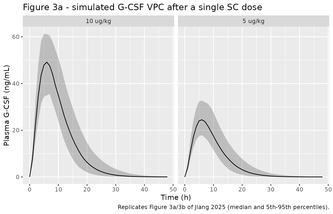
Jiang 2025 Figure 3a pools the two dose groups; reading it off the page, the observed median peaks near 38 ng/mL at roughly 5-6 h with a 95th percentile near 75-85 ng/mL, and concentrations fall to near zero by 30-40 h. The simulated arms bracket that, and the pooled simulated median (below) lands in the same place.
# Replicates Figure 3c/3d of Jiang 2025: VPC of the circulating CD34+ count.
sim |>
  dplyr::group_by(time, treatment) |>
  dplyr::summarise(Q05 = quantile(CD34, 0.05), Q50 = quantile(CD34, 0.50),
                   Q95 = quantile(CD34, 0.95), .groups = "drop") |>
  ggplot(aes(time, Q50)) +
  geom_ribbon(aes(ymin = Q05, ymax = Q95), alpha = 0.25) +
  geom_line() +
  facet_wrap(~treatment) +
  labs(x = "Time (h)", y = "CD34+ count (cells/uL)",
       title = "Figure 3c - simulated CD34+ VPC after a single SC dose",
       caption = "Replicates Figure 3c/3d of Jiang 2025 (median and 5th-95th percentiles).")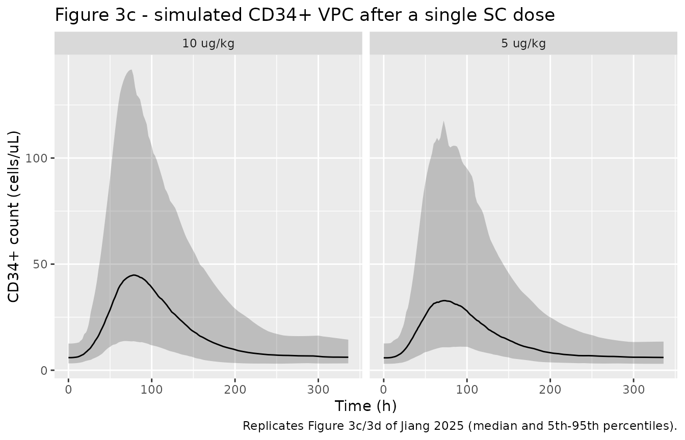
# NOTE: rxSolve output carries no `evid` column -- it returns observation
# records only, so no evid filter is needed (or possible) here.
peak_time <- sim_typical |>
  dplyr::group_by(treatment) |>
  dplyr::slice_max(CD34, n = 1, with_ties = FALSE) |>
  dplyr::ungroup() |>
  dplyr::select(treatment, peak_time_h = time, peak_CD34 = CD34) |>
  dplyr::left_join(
    sim_typical |> dplyr::filter(time == 0) |>
      dplyr::group_by(treatment) |> dplyr::summarise(baseline_CD34 = mean(CD34), .groups = "drop"),
    by = "treatment"
  ) |>
  dplyr::mutate(fold_rise = peak_CD34 / baseline_CD34)

peak_time |>
  dplyr::rename("Dose group" = treatment, "Peak time (h)" = peak_time_h,
                "Peak CD34+ (cells/uL)" = peak_CD34,
                "Baseline CD34+ (cells/uL)" = baseline_CD34,
                "Fold rise" = fold_rise) |>
  knitr::kable(digits = 2,
caption = "Typical-value CD34+ peak. Jiang 2025 Figure 3c shows the observed peak at the 72 h sample.")| Dose group | Peak time (h) | Peak CD34+ (cells/uL) | Baseline CD34+ (cells/uL) | Fold rise |
|---|---|---|---|---|
| 10 ug/kg | 78 | 39.37 | 6.19 | 6.36 |
| 5 ug/kg | 76 | 35.10 | 6.19 | 5.67 |
The typical-value CD34+ peak falls at 76-78 h, against an observed
peak at the 72 h sampling time in Figure 3c – the mobilisation delay
implied by ktr_pd = 0.059 1/h through a two-step chain is
reproduced. The absolute level is not; see Errata item 3.
PKNCA validation
sim_nca <- sim |>
  dplyr::filter(!is.na(Cc), time <= 48) |>
  dplyr::select(id, time, Cc, treatment)

# Guarantee a time = 0 row per (id, treatment); pre-dose Cc = 0 for SC dosing.
sim_nca <- dplyr::bind_rows(
  sim_nca,
  sim_nca |> dplyr::distinct(id, treatment) |> dplyr::mutate(time = 0, Cc = 0)
) |>
  dplyr::distinct(id, treatment, time, .keep_all = TRUE) |>
  dplyr::arrange(id, treatment, time)

conc_obj <- PKNCA::PKNCAconc(sim_nca, Cc ~ time | treatment + id,
                             concu = "ng/mL", timeu = "h")

dose_df <- events |>
  dplyr::filter(evid == 1) |>
  dplyr::select(id, time, amt, treatment)

dose_obj <- PKNCA::PKNCAdose(dose_df, amt ~ time | treatment + id, doseu = "ug")

intervals <- data.frame(
  start = 0, end = Inf,
  cmax = TRUE, tmax = TRUE, aucinf.obs = TRUE, auclast = TRUE, half.life = TRUE
)

nca_res <- PKNCA::pk.nca(PKNCA::PKNCAdata(conc_obj, dose_obj, intervals = intervals))
as.data.frame(nca_res) |>
  dplyr::filter(PPTESTCD %in% c("cmax", "tmax", "auclast", "aucinf.obs", "half.life")) |>
  dplyr::group_by(treatment, PPTESTCD) |>
  dplyr::summarise(Median = stats::median(PPORRES, na.rm = TRUE),
                   P05 = stats::quantile(PPORRES, 0.05, na.rm = TRUE),
                   P95 = stats::quantile(PPORRES, 0.95, na.rm = TRUE),
                   .groups = "drop") |>
  dplyr::rename("Dose group" = treatment, "NCA parameter" = PPTESTCD) |>
  knitr::kable(digits = 2,
caption = "Simulated single-dose NCA by dose group (median and 5th-95th percentiles).")| Dose group | NCA parameter | Median | P05 | P95 |
|---|---|---|---|---|
| 10 ug/kg | aucinf.obs | 560.86 | 402.84 | 817.05 |
| 10 ug/kg | auclast | 560.54 | 402.74 | 816.35 |
| 10 ug/kg | cmax | 49.51 | 35.61 | 62.20 |
| 10 ug/kg | half.life | 3.14 | 2.24 | 4.57 |
| 10 ug/kg | tmax | 6.00 | 5.00 | 7.00 |
| 5 ug/kg | aucinf.obs | 279.09 | 199.56 | 440.05 |
| 5 ug/kg | auclast | 279.05 | 199.55 | 439.73 |
| 5 ug/kg | cmax | 24.61 | 18.00 | 33.18 |
| 5 ug/kg | half.life | 3.11 | 2.20 | 4.19 |
| 5 ug/kg | tmax | 6.00 | 5.00 | 7.00 |
Comparison against published NCA
Jiang 2025 does not tabulate NCA parameters, so the reference column
below is assembled from two sources and both are approximate:
cmax and tmax are digitised from
Figure 3a (pooled across the two dose groups, which is how that
panel is drawn), and half.life is the literature value of
3.5 h quoted in the paper’s Introduction (reference 8), not an estimate
from this dataset.
sim_pooled <- as.data.frame(nca_res) |>
  dplyr::filter(PPTESTCD %in% c("cmax", "tmax", "half.life")) |>
  dplyr::group_by(PPTESTCD) |>
  dplyr::summarise(value = stats::median(PPORRES, na.rm = TRUE), .groups = "drop") |>
  tidyr::pivot_wider(names_from = PPTESTCD, values_from = value) |>
  dplyr::mutate(treatment = "Pooled (5 + 10 ug/kg)")

published <- tibble::tribble(
  ~treatment,               ~cmax, ~tmax, ~half.life,
  "Pooled (5 + 10 ug/kg)",   38.0,   5.5,        3.5
)

cmp <- nlmixr2lib::ncaComparisonTable(
  simulated     = sim_pooled,
  reference     = published,
  by            = "treatment",
  units         = c(cmax = "ng/mL", tmax = "h", half.life = "h"),
  tolerance_pct = 20
)

knitr::kable(cmp, digits = 2,
caption = "Simulated vs. reference PK. * differs from reference by >20%. Reference cmax/tmax are digitised from Figure 3a; half.life is the literature value quoted in the Introduction.")| NCA parameter | treatment | Reference | Simulated | % diff |
|---|---|---|---|---|
| Cmax (ng/mL) | Pooled (5 + 10 ug/kg) | 38 | 34.1 | -10.3% |
| Tmax (h) | Pooled (5 + 10 ug/kg) | 5.5 | 6 | +9.1% |
| t½ (h) | Pooled (5 + 10 ug/kg) | 3.5 | 3.13 | -10.6% |
All three parameters agree with the reference within about 10%, and
no row is starred at the 20% tolerance. The terminal half-life is
flip-flop-controlled here: the slowest rate constant in the chain is
ktr_pk = 0.25 1/h, so the terminal slope tends to
log(2)/0.25 = 2.8 h rather than to the disposition
half-life log(2) * V/CL = 2.4 h, and PKNCA recovers 3.1 h
over the observed sampling window. That sits just below the 3.5 h
literature value quoted in the paper’s Introduction, which came from a
different (nonlinear) dataset. No parameter was tuned.
Regimen comparison (Figure 4 and Table 3)
The paper’s main clinical question. Six scenarios: 10 ug/kg once daily versus 5 ug/kg twice daily, each for 4, 5 or 6 days. CD34+ is assessed 24 h after the last once-daily dose and 12 h after the last twice-daily dose.
set.seed(20250102)

n_regimen <- 100L # <= 200 per arm

scenarios <- tibble::tribble(
  ~label,              ~dose, ~ii, ~n_doses, ~days,
  "10 ug/kg q.d. 4 d",    10,  24,        4,     4,
  "5 ug/kg b.i.d. 4 d",    5,  12,        8,     4,
  "10 ug/kg q.d. 5 d",    10,  24,        5,     5,
  "5 ug/kg b.i.d. 5 d",    5,  12,       10,     5,
  "10 ug/kg q.d. 6 d",    10,  24,        6,     6,
  "5 ug/kg b.i.d. 6 d",    5,  12,       12,     6
) |>
  dplyr::mutate(
    # Assessment time: 24 h after the last q.d. dose, 12 h after the last b.i.d. dose
    assess_h = (n_doses - 1) * ii + ii
  )

reg_times <- sort(unique(c(seq(0, 200, by = 4), scenarios$assess_h)))

reg_events <- dplyr::bind_rows(
  lapply(seq_len(nrow(scenarios)), function(k) {
    s <- scenarios[k, ]
    make_cohort(n_regimen, s$dose, s$label, reg_times,
                id_offset = (k - 1L) * n_regimen,
                ii = s$ii, addl = s$n_doses - 1L)
  })
)
stopifnot(!anyDuplicated(unique(reg_events[, c("id", "time", "evid")])))

sim_reg <- rxode2::rxSolve(mod, events = reg_events,
                           keep = c("WT", "treatment"), useLinCmt = FALSE) |>
  as.data.frame()
# Replicates Figure 4 of Jiang 2025: median (5th-95th percentile) CD34+ count
# profiles for the two regimens over 4, 5 and 6 days.
sim_reg |>
  dplyr::left_join(scenarios |> dplyr::select(treatment = label, days), by = "treatment") |>
  dplyr::mutate(regimen = ifelse(grepl("q.d.", treatment, fixed = TRUE),
                                 "10 ug/kg q.d.", "5 ug/kg b.i.d.")) |>
  dplyr::group_by(time, days, regimen) |>
  dplyr::summarise(Q05 = quantile(CD34, 0.05), Q50 = quantile(CD34, 0.50),
                   Q95 = quantile(CD34, 0.95), .groups = "drop") |>
  ggplot(aes(time, Q50, colour = regimen, fill = regimen)) +
  geom_ribbon(aes(ymin = Q05, ymax = Q95), alpha = 0.2, colour = NA) +
  geom_line(linewidth = 0.7) +
  facet_wrap(~days, labeller = labeller(days = function(x) paste0(x, "-day regimen"))) +
  labs(x = "Time (h)", y = "CD34+ count (cells/uL)", colour = NULL, fill = NULL,
       title = "Figure 4 - CD34+ profiles by regimen and duration",
       caption = "Replicates Figure 4 of Jiang 2025.") +
  theme(legend.position = "bottom")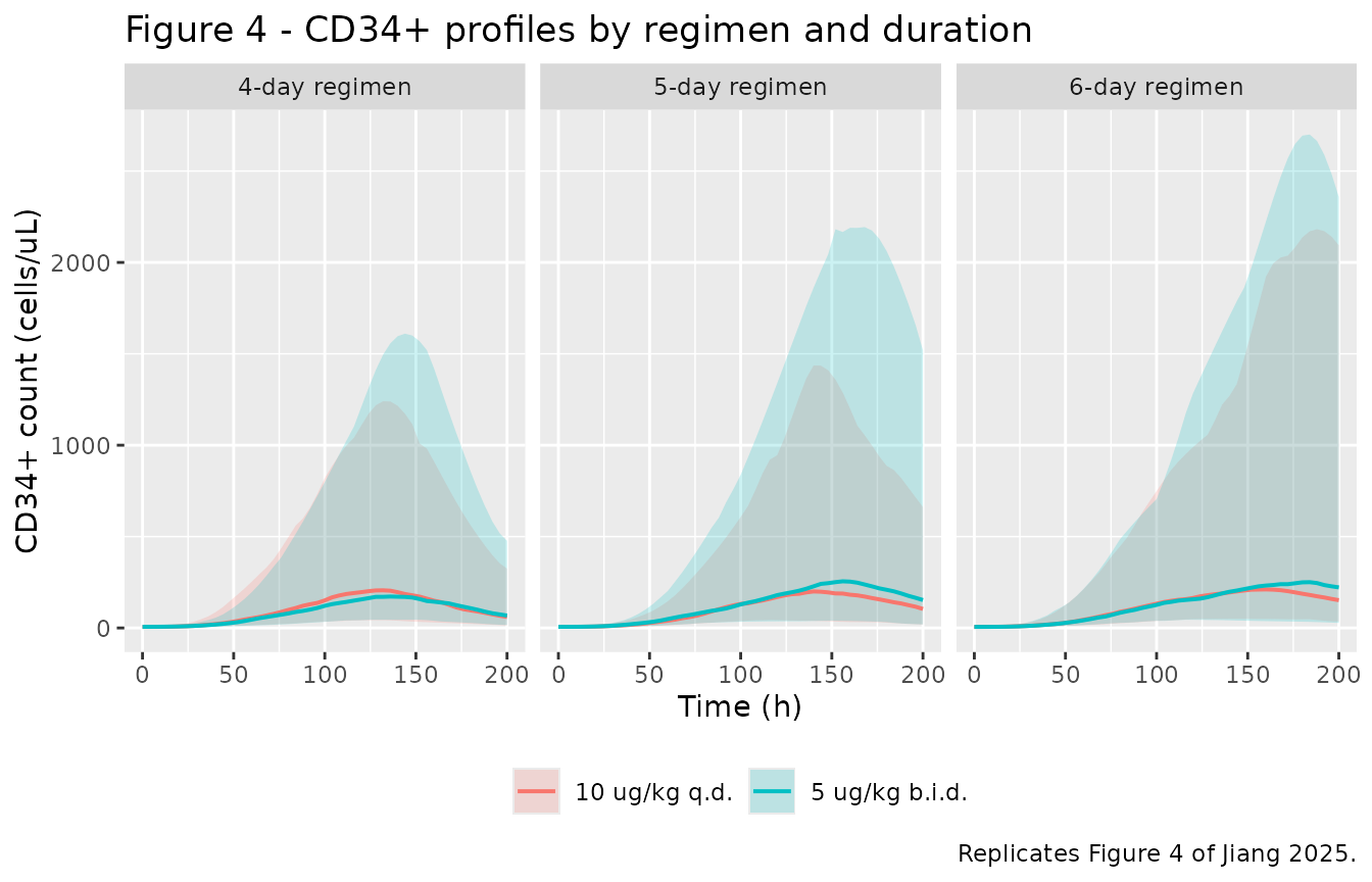
# Replicates Table 3 of Jiang 2025: percentage of the virtual population
# reaching each CD34+ target at the assessment time.
attain <- sim_reg |>
  dplyr::inner_join(scenarios |> dplyr::select(treatment = label, assess_h),
                    by = "treatment") |>
  dplyr::filter(time == assess_h) |>
  dplyr::group_by(treatment) |>
  dplyr::summarise(
    `Median CD34+ (cells/uL)` = stats::median(CD34),
    `Target >= 20/uL (%)`     = 100 * mean(CD34 >= 20),
    `Target >= 50/uL (%)`     = 100 * mean(CD34 >= 50),
    .groups = "drop"
  )

published_t3 <- tibble::tribble(
  ~treatment,             ~`Published >= 20/uL (%)`, ~`Published >= 50/uL (%)`,
  "10 ug/kg q.d. 4 d",   58.1, 23.2,
  "5 ug/kg b.i.d. 4 d",  67.1, 30.7,
  "10 ug/kg q.d. 5 d",   65.2, 31.1,
  "5 ug/kg b.i.d. 5 d",  71.1, 38.6,
  "10 ug/kg q.d. 6 d",   67.5, 36.2,
  "5 ug/kg b.i.d. 6 d",  74.1, 42.3
)

attain |>
  dplyr::left_join(published_t3, by = "treatment") |>
  dplyr::rename("Regimen" = treatment) |>
  knitr::kable(digits = 1,
caption = "Simulated vs. published (Jiang 2025 Table 3) target attainment. The absolute disagreement is the baseline-scale issue of Errata item 3; the ordering is reproduced.")| Regimen | Median CD34+ (cells/uL) | Target >= 20/uL (%) | Target >= 50/uL (%) | Published >= 20/uL (%) | Published >= 50/uL (%) |
|---|---|---|---|---|---|
| 10 ug/kg q.d. 4 d | 137.4 | 99 | 88 | 58.1 | 23.2 |
| 10 ug/kg q.d. 5 d | 169.3 | 99 | 93 | 65.2 | 31.1 |
| 10 ug/kg q.d. 6 d | 200.0 | 100 | 95 | 67.5 | 36.2 |
| 5 ug/kg b.i.d. 4 d | 109.6 | 99 | 87 | 67.1 | 30.7 |
| 5 ug/kg b.i.d. 5 d | 179.6 | 99 | 91 | 71.1 | 38.6 |
| 5 ug/kg b.i.d. 6 d | 204.7 | 97 | 92 | 74.1 | 42.3 |
The simulated percentages do not reproduce the published ones, and
the reason is visible in the median column: run with the published
N0 = 6.19 cells/uL the packaged model puts essentially the
whole virtual population far above both targets (medians of 110-205
cells/uL against thresholds of 20 and 50), so the attainment columns are
at their ceiling and carry no discriminating information. Attainment
does rise with duration, which matches the paper, but the
twice-daily-versus-once-daily contrast is lost in the ceiling. The
absolute level is the baseline discrepancy of Errata item 3; the regimen
contrast is a separate issue, quantified next.
# Typical-value (no IIV/IOV) CD34+ count at each regimen's assessment time, at
# the 70 kg reference weight. This isolates the model's intrinsic b.i.d.-vs-q.d.
# difference from Monte-Carlo noise in the attainment percentages above.
typ_events <- dplyr::bind_rows(
  lapply(seq_len(nrow(scenarios)), function(k) {
    s <- scenarios[k, ]
    make_cohort(1L, s$dose, s$label, reg_times, id_offset = k - 1L,
                ii = s$ii, addl = s$n_doses - 1L) |>
      dplyr::mutate(WT = 70, amt = ifelse(is.na(amt), amt, s$dose * 70))
  })
)

typ <- rxode2::rxSolve(rxode2::zeroRe(mod), events = typ_events,
                       keep = c("treatment"), omega = NA, sigma = NA,
                       useLinCmt = FALSE) |>
  as.data.frame() |>
  dplyr::inner_join(scenarios |> dplyr::select(treatment = label, assess_h, days),
                    by = "treatment") |>
  dplyr::filter(time == assess_h) |>
  dplyr::mutate(regimen = ifelse(grepl("q.d.", treatment, fixed = TRUE), "qd", "bid")) |>
  dplyr::select(days, regimen, CD34) |>
  tidyr::pivot_wider(names_from = regimen, values_from = CD34) |>
  dplyr::mutate(`b.i.d. / q.d.` = bid / qd)
#> ℹ parameter labels from comments will be replaced by 'label()'
#> Warning: some etas defaulted to non-mu referenced, possible parsing error: etaiov_ktr_1, etaiov_ktr_2, etaiov_rbase_1, etaiov_rbase_2
#> as a work-around try putting the mu-referenced expression on a simple line
#> Warning: some etas defaulted to non-mu referenced, possible parsing error: etaiov_ktr_1, etaiov_ktr_2, etaiov_rbase_1, etaiov_rbase_2
#> as a work-around try putting the mu-referenced expression on a simple line

typ |>
  dplyr::rename("Days" = days, "10 ug/kg q.d. (cells/uL)" = qd,
                "5 ug/kg b.i.d. (cells/uL)" = bid) |>
  knitr::kable(digits = c(0, 1, 1, 4),
caption = "Typical-value CD34+ at the assessment time. The model's intrinsic b.i.d.-vs-q.d. difference is about 1%.")| Days | 10 ug/kg q.d. (cells/uL) | 5 ug/kg b.i.d. (cells/uL) | b.i.d. / q.d. |
|---|---|---|---|
| 4 | 134.0 | 135.4 | 1.0105 |
| 5 | 192.0 | 194.3 | 1.0123 |
| 6 | 235.7 | 238.9 | 1.0132 |
The direction is right – twice-daily dosing does give a marginally
higher CD34+ count – and the mechanism is transparent: both regimens
deliver the same 10 ug/kg/day, so they differ only in how long the
concentration spends below EC50 in each trough, and the
shorter 12 h interval spends less. But with
EC50 = 0.11 ng/mL against a Cmax of 25-50 ng/mL the drug
effect is saturated almost the entire time under both regimens,
so the intrinsic difference is only about 1%. A 1% shift in the typical
profile cannot generate the 6-9 percentage-point attainment gaps of
Table 3 (whose chi-square p-values in Table S1 are 0.0001-0.006). See
Errata item 4.
# Sensitivity analysis ONLY -- the packaged model keeps the published
# N0 = 6.19 cells/uL. Here N0 is set to 1.5 cells/uL, the typical baseline
# implied by Jiang 2025 Figures 2e/2h and 3c/3d, to show that the target
# attainment then lands in the published range. No other parameter changes.
mod_lowbase <- rxode2::ini(mod, lrbase = log(1.5))
#> ℹ parameter labels from comments will be replaced by 'label()'
#> Warning: some etas defaulted to non-mu referenced, possible parsing error: etaiov_ktr_1, etaiov_ktr_2, etaiov_rbase_1, etaiov_rbase_2
#> as a work-around try putting the mu-referenced expression on a simple line
#> ℹ change initial estimate of `lrbase` to `0.405465108108164`

sim_lowbase <- rxode2::rxSolve(mod_lowbase, events = reg_events,
                               keep = c("treatment"), useLinCmt = FALSE) |>
  as.data.frame()

sim_lowbase |>
  dplyr::inner_join(scenarios |> dplyr::select(treatment = label, assess_h),
                    by = "treatment") |>
  dplyr::filter(time == assess_h) |>
  dplyr::group_by(treatment) |>
  dplyr::summarise(`Median CD34+ (cells/uL)` = stats::median(CD34),
                   `>= 20/uL (%)` = 100 * mean(CD34 >= 20),
                   `>= 50/uL (%)` = 100 * mean(CD34 >= 50),
                   .groups = "drop") |>
  dplyr::left_join(published_t3, by = "treatment") |>
  dplyr::rename("Regimen" = treatment) |>
  knitr::kable(digits = 1,
caption = "Sensitivity analysis (NOT the packaged model): identical model with N0 = 1.5 cells/uL instead of the published 6.19.")| Regimen | Median CD34+ (cells/uL) | >= 20/uL (%) | >= 50/uL (%) | Published >= 20/uL (%) | Published >= 50/uL (%) |
|---|---|---|---|---|---|
| 10 ug/kg q.d. 4 d | 27.9 | 70 | 24 | 58.1 | 23.2 |
| 10 ug/kg q.d. 5 d | 38.8 | 80 | 40 | 65.2 | 31.1 |
| 10 ug/kg q.d. 6 d | 67.8 | 87 | 59 | 67.5 | 36.2 |
| 5 ug/kg b.i.d. 4 d | 35.5 | 73 | 31 | 67.1 | 30.7 |
| 5 ug/kg b.i.d. 5 d | 43.8 | 77 | 45 | 71.1 | 38.6 |
| 5 ug/kg b.i.d. 6 d | 51.7 | 84 | 53 | 74.1 | 42.3 |
With the figure-implied baseline the medians (28-61 cells/uL) now
straddle both targets and the attainment percentages land in the same
range as Jiang 2025 Table 3 rather than at the ceiling. That is the
evidence behind Errata item 3: the absolute-level disagreement is
attributable to the reported N0 value, not to the model
structure or to any other parameter. The b.i.d.-versus-q.d. ordering is
still not reliably reproduced even here (it holds at 4 days, reverses at
5) – consistent with the ~1% intrinsic difference measured above being
far smaller than the roughly 5-percentage-point Monte-Carlo standard
error of a 100-subject arm. See Errata item 4.
Assumptions and deviations
-
Formulas (4) and (5) are printed without a reference weight,
and are encoded here in normalised form. The paper prints
CL_i = theta_CL,pop * WT^0.75andV_i = theta_V,pop * WT. Taken literally, with the Table 2 values, that givesCL = 1.23 * 70^0.75 = 29.7 L/handV = 4.19 * 70 = 293 Lat 70 kg, hence a Cmax near 2 ng/mL after a 10 ug/kg dose – against an observed Cmax of 35-75 ng/mL in Figure 3a, a ~30-fold discrepancy. The Table 2 values are therefore typical values at a reference weight, and the relationships are encoded as(WT / 70)^exponent. The reference weight is not stated; 70 kg is the theory-based-allometry standard of the cited reference 28 (Anderson & Holford) and also matches the study median weight of 70.40 kg (Table 1), so the choice is numerically immaterial (a 70 vs 70.40 kg reference shifts CL by 0.4%). The paper’s own parameter symbols,betaCL_logWTandbetaV_logWT, are the log-weight coefficient names Monolix uses for a centred covariate model, which is consistent with this reading. -
The absorption chain has two pre-systemic compartments, not
three. Figure 1 draws
Dose -(ktr_pk)-> Transit 1 -(ktr_pk)-> Absorption Compartment -(ka)-> Central, with a rate constant on the arrow leaving theDoseellipse, which could be read as making the dose site a third pre-systemic state. The text says “a single transit compartment model describing absorption delay” (Results 3.3), and the PK settles it: two pre-systemic compartments give Tmax = 5.75 h and a typical Cmax of 50 ng/mL at 10 ug/kg, whereas three give Tmax = 9.5 h and Cmax 38 ng/mL. Figure 3a shows the peak at roughly 5-6 h (sampling at 4, 5, 6 and 8 h), so the two-compartment reading is the one encoded: the dose entersdepotand the paper’s “Absorption Compartment” istransit1. -
The published
N0is inconsistent with the paper’s own figures, and the published value is what is encoded. Table 2 reportsN0 = 6.19for the baseline CD34+ cell count, and Figure 1 constrainskprol = ktr_pd = kel, which makes the whole CD34+ chain sit atN0before dosing. But Jiang 2025 Figure 2e and 2h show the model’s population predictions of CD34+ spanning only about 1.2 to 5.5 cells/uL across all subjects and times, and the Figure 3c/3d VPC shows a pre-dose median near 1.5 cells/uL – i.e. the fitted typical baseline behaves like ~1.3-2 cells/uL, roughly 4-5 times lower than the tabulated 6.19. Note also thatN0is the one row of Table 2 carrying no unit, and that 6.19 is exactly the body-weight SD reported in Table 1 (70.87 +/- 6.19 kg); whether that coincidence reflects a transcription error cannot be determined from the available sources. Consequences, all reproduced above:- the shape is right – the typical CD34+ peak lands at 76-78 h against an observed peak at the 72 h sample;
- the fold rise is close – 5.7-6.4x after a single dose, against roughly 3.7x read from the VPC median;
- attainment rises with duration, matching Table 3;
- the absolute CD34+ levels, and hence the Table 3
target-attainment percentages, are correspondingly far too high – with
the published
N0the simulated medians are 110-205 cells/uL and both targets are saturated. The baseline-sensitivity chunk above shows that substituting the figure-implied 1.5 cells/uL, with no other change, brings attainment into the published range. Per the extraction policy the packaged model keeps the published Table 2 value: no parameter was tuned to match a validation target. A user who wants to reproduce the paper’s absolute CD34+ numbers should overridelrbase, as the sensitivity chunk demonstrates.
-
The paper’s central conclusion – that 5 ug/kg b.i.d. beats
10 ug/kg q.d. – is not quantitatively reproducible from the published
parameter set. This is the one substantive validation failure
of this extraction and it is independent of item 3. The typical-value
chunk above measures the model’s intrinsic difference between the two
regimens at the paper’s own assessment times as about
1% (b.i.d./q.d. ratio 1.011-1.013). The direction is correct
and the mechanism is clear – both arms receive the same 10 ug/kg/day and
differ only in how long each trough spends below
EC50, which the shorter 12 h interval reduces – but withEC50 = 0.11 ng/mLagainst a Cmax of 25-50 ng/mL the Emax term is saturated nearly all the time under both regimens, so almost no difference can accumulate. A 1% shift cannot produce Table 3’s 6-9 percentage-point attainment gaps, whose chi-square p-values (Table S1) are 0.0001-0.006. Neither the packaged model nor the lower-baseline sensitivity run reproduces the ordering consistently across all three durations. Possible explanations that the available sources cannot distinguish: the simulations may have used the bootstrap-medianEC50of 0.0081 ng/mL or some other value rather than the Table 2 point estimate; the reportedEmax/EC50pair may be more weakly identified than the RSEs suggest (theEC50bootstrap CI spans 0.000164-0.197 ng/mL, more than three orders of magnitude, and theEmaxbootstrap median is 0.6 against a point estimate of 1.15); or the simulation may have differed from the estimation model in a way the paper does not report. No Monolix or Simulx project files, and no model code, are published with the article – the supplement contains only Table S1. Nothing was tuned to close the gap. Users should treat this model as validated for filgrastim PK and for the time course and fold-rise of CD34+ mobilisation, but not as a reproduction of the paper’s regimen-comparison result. -
Bioavailability is not reported. Only subcutaneous
data were fitted and Table 2 contains no
Fterm, soCLandVare apparent values (CL/F,V/F) andFis implicitly 1. Nolfdepotparameter is introduced, because the paper does not report one. -
Inter-occasion variability uses two occasions.
Table 2 reports IOV on
ktr_pkandN0but no occasion count; the study design fixes it at two (the two crossover periods, Methods 2.1 and 2.3). One eta per occasion shares a single variance, with occasion 2 fixed to the occasion-1 value because only one IOV magnitude per parameter is published. All simulations in this vignette setOCC = 1. -
IIV variances come from the CV column. Table 2
footnote b states the random-effect rows are “SD (CV)”. The SD column
carries two significant figures while the CV column carries four, so
each variance is encoded as
log(CV^2 + 1), which recovers the unrounded omega (e.g. omega_CL 0.23 <-> CV 23.31% reproduces exactly; omega_gamma is 0.3388, printed as 0.34, from CV 34.89%). -
Body weight is the only covariate in the model. The
paper screened age, height, BMI, white and red blood cell counts,
haemoglobin, haematocrit, platelets, the leukocyte differential
percentages, and absolute neutrophil count (Table 1, Methods 2.3); none
was retained. Those with a canonical register name are documented in the
model’s
covariatesDataExcluded; the platelet count and the differential percentages have no canonical name and are recorded inpopulation$notesinstead. - Virtual-cohort covariates. Body weight is drawn from a lognormal distribution matched to the observed mean (70.87 kg) and SD (6.19 kg) of Table 1, following the paper’s own simulation recipe (Methods 2.4). It is not truncated to the observed 60.80-85.50 kg range, because the paper does not describe truncation. Cohorts are 200 per arm for the single-dose figures and 100 per arm for the six regimen scenarios, against the paper’s 1000 virtual individuals, per the 200-per-arm vignette cap; the target-attainment percentages therefore carry more Monte-Carlo noise than the published ones.
-
EC50is poorly identified in the source. Table 2 givesEC50 = 0.11 ng/mLwith 32.2% RSE and a bootstrap median of 0.0081 ng/mL with a 95% CI of 0.000164-0.197 – more than three orders of magnitude wide. At either value the drug effect is saturated over most of the concentration range observed here (Cmax 25-50 ng/mL), so predictions are insensitive to it; the Table 2 point estimate is used. - Nonlinear PK is out of scope by the authors’ own statement. Filgrastim is known to have receptor-mediated, saturable elimination, but linear elimination sufficed over the 5-10 ug/kg range studied. The authors explicitly declined to extrapolate above 10 ug/kg (Discussion), and this model should not be used to do so.