Sotatercept (Ait-Oudhia 2024)
Source:vignettes/articles/AitOudhia_2024_sotatercept.Rmd
AitOudhia_2024_sotatercept.RmdModel and source
- Citation: Ait-Oudhia S, Jaworowicz D, Hu Z, Bihorel S, Hu S, Balasubrahmanyam B, Mistry B, de Oliveira Pena J, Wenning L, Gheyas F. Population pharmacokinetic modeling of sotatercept in healthy participants and patients with pulmonary arterial hypertension. CPT Pharmacometrics Syst Pharmacol. 2024;13(8):1380-1393. doi:10.1002/psp4.13166
- Description: Two-compartment population pharmacokinetic model for sotatercept in healthy post-menopausal women and patients with pulmonary arterial hypertension (Ait-Oudhia 2024). First-order subcutaneous absorption with logit-scale bioavailability (about 66%) and linear elimination from the central compartment; time-varying body weight enters as a power covariate on clearance (exponent 0.814) and central volume (exponent 1.02) with a 70 kg reference, and baseline serum albumin as a power covariate on clearance (exponent -0.849) with a 4.5 g/dL reference. Separate log-scale residual error magnitudes are used for healthy participants and for patients with PAH. Intravenous doses go to the central compartment and subcutaneous doses to the depot.
- Article: https://doi.org/10.1002/psp4.13166
Sotatercept is a first-in-class recombinant fusion protein (the extracellular domain of activin receptor type IIA linked to a human IgG1 Fc domain) approved for pulmonary arterial hypertension (PAH). Ait-Oudhia 2024 pooled five trials into one integrated population PK model: a two-compartment model with first-order subcutaneous (SC) absorption, linear elimination from the central compartment, and time-varying body weight plus baseline serum albumin as the two retained covariates.
Population
The final analysis dataset comprised 350 participants: 40 from a phase 1 single-ascending-dose (SAD) trial and 24 from a phase 1 multiple-ascending-dose (MAD) trial, both in healthy post-menopausal women, plus 103 from PULSAR, 21 from SPECTRA (phase 2), and 162 from STELLAR (phase 3), all in participants with PAH (Table 1). 30 participants received sotatercept intravenously (IV) and 320 subcutaneously.
Participants were 85.1% female (298 of 350) – both phase 1 trials enrolled only post-menopausal women – with a mean age of 50.2 years (SD 14.4, range 18-81) and a mean baseline body weight of 71.0 kg (SD 17.6, range 39.6-136). Mean baseline serum albumin was 4.43 g/dL (SD 0.33, range 2.9-5.8), i.e. 44.3 g/L (range 29-58) in the SI units this package uses. 82.9% self-identified as White/Caucasian, 7.14% Asian, 3.14% Black or African American, 1.14% Native Hawaiian or other Pacific Islander, 0.286% American Indian or Alaska Native, and 5.43% Other. Renal function at baseline was normal in 33.1%, mildly impaired in 52.3%, and moderately impaired in 14.6%; severe impairment (eGFR below 30 mL/min/1.73 m^2) was an exclusion criterion (Table 1).
Doses spanned single IV or SC 0.01-3.0 mg/kg (SAD) and multiple SC 0.03-1.0 mg/kg Q4W (MAD) in phase 1, SC 0.3 or 0.7 mg/kg Q3W in phase 2, and an SC 0.3 mg/kg initial dose followed by the 0.7 mg/kg Q3W target dose in phase 3. PK sampling was rich in the two phase 1 studies and sparse in phase 2/3, with samples collected for up to about 150 weeks (Figure 1).
The same information is available programmatically via the model’s
population metadata
(readModelDb("AitOudhia_2024_sotatercept")()$population).
Source trace
The per-parameter origin is recorded as an in-file comment next to
each ini() entry in
inst/modeldb/specificDrugs/AitOudhia_2024_sotatercept.R.
The table below collects them in one place for review. All values come
from Table 2 of Ait-Oudhia 2024; every parameter was estimated (each
carries a %RSE), so none is wrapped in fixed().
| Equation / parameter | Value | Source location |
|---|---|---|
lcl (CL) |
0.177 L/day | Table 2, CL population mean (%RSE 6.22) |
lvc (VC) |
3.60 L | Table 2, VC population mean (%RSE 5.50) |
lq (Q) |
0.487 L/day | Table 2, Q population mean (%RSE 20.5) |
lvp (VP) |
1.71 L | Table 2, VP population mean (%RSE 15.8) |
lka (KA) |
0.273 1/day | Table 2, KA population mean (%RSE 16.0) |
logitfdepot (F1) |
logit(0.659) = 0.6588 | Table 2, F1 population mean (%RSE 6.29) |
e_wt_cl |
0.814 | Table 2, CL “Exponent of body weight power effect” (%RSE 11.9) |
e_alb_cl |
-0.849 | Table 2, CL “Exponent of baseline albumin effect” (%RSE 24.2) |
e_wt_vc |
1.02 | Table 2, VC “Exponent of body weight power effect” (%RSE 11.8) |
etalcl |
log(1 + 0.283^2) = 0.0770 | Table 2, CL IIV 28.3 %CV; Methods %CV = sqrt(exp(omega^2) - 1) x 100 |
etalvc |
log(1 + 0.247^2) = 0.0592 | Table 2, VC IIV 24.7 %CV |
etalvp |
log(1 + 0.733^2) = 0.4300 | Table 2, VP IIV 73.3 %CV |
etalka |
log(1 + 0.604^2) = 0.3110 | Table 2, KA IIV 60.4 %CV |
etalogitfdepot |
0.348^2 = 0.1211 | Table 2, F1 IIV 11.9 %CV via footnote d: 100 x (1 - 0.659) x 0.348 |
| (no IIV on Q) | n/a | Table 2 reports “NE” (not estimated) in the Q variability column |
expSdHealthy |
sqrt(0.0570) = 0.2387 | Table 2, “Residual variability in HV (log units)” variance (%RSE 20.2); reported SD 0.239 |
expSdPah |
sqrt(0.0357) = 0.1889 | Table 2, “Residual variability in PAH (log units)” variance (%RSE 12.6); reported SD 0.189 |
| CL covariate equation | CL = 0.177 x (WT/70)^0.814 x (ALB/45)^-0.849 |
Table 2 footnote a (printed with a 4.5 g/dL albumin reference; see Assumptions) |
| VC covariate equation | VC = 3.60 x (WT/70)^1.02 |
Table 2 footnote c |
| Micro-constants |
k12 = Q/VC, k21 = Q/VP,
kel = CL/VC
|
Methods, “Clinical relevance of covariates” (t-half derivation) |
| Two-compartment ODEs with SC depot | n/a | Figure 2 schematic; Methods, “Data analyses and population pharmacokinetic modeling approach” |
| Residual error form |
log(Y) = log(Yhat) + eps (nlmixr2
lnorm) |
Methods, “Log error model”; Results, “Two separate log error models … for healthy and PAH participants” |
Validation strategy
Ait-Oudhia 2024 publishes no non-compartmental analysis table, so this vignette validates against the derived quantities the paper does report. Four of these are exact, independent checks on the packaged model:
- Terminal half-life about 22 days for a typical 70 kg participant with a median normal baseline albumin of 4.5 g/dL (Discussion). This is an end-to-end gate: it depends jointly on CL, VC, Q, and VP.
- Typical CL of 0.135, 0.177, and 0.237 L/day and typical VC of 2.55, 3.60, and 5.18 L at body weights of 50, 70, and 100 kg (Discussion). This pins both weight exponents and both reference values.
- SC bioavailability of about 66%, recoverable as the SC-to-IV AUC ratio (Table 2, Abstract).
- Dose-proportional PK across all studied doses (“At all studied doses, sotatercept PK appeared to be linear as assessed by the dose-normalized exposure data”, Discussion).
A fifth, softer check is the paper’s statement of “an observed 35% variability in sotatercept AUC” (Discussion), compared below against the model-predicted between-subject variability in steady-state AUC.
Deterministic gates
These use omega = NA to suppress between-subject
variability, so each solve returns the typical-value profile.
(omega = NA is preferred over
rxode2::zeroRe(), which mutates shared model state.)
mod <- readModelDb("AitOudhia_2024_sotatercept")

# Typical individual: 70 kg, albumin 45 g/L (= 4.5 g/dL), PAH cohort.
solve_typical <- function(events, wt = 70, alb = 45, healthy = 0) {
  d <- as.data.frame(events)
  d$WT <- wt
  d$ALB <- alb
  d$DIS_HEALTHY <- healthy
  # steady-state searches for long-half-life subjects exceed the default step budget
  rxode2::rxSolve(mod, d, omega = NA, returnType = "data.frame", maxsteps = 1e6)
}
Gate 2 – typical CL and VC versus body weight
probe <- rxode2::et(amt = 49, cmt = "depot") |>
  rxode2::et(0, cmt = "central")

wt_gate <- lapply(c(50, 70, 100), function(w) {
  s <- solve_typical(probe, wt = w)
  tibble(WT = w, cl_model = s$cl[1], vc_model = s$vc[1])
}) |>
  bind_rows() |>
  mutate(
    cl_paper = c(0.135, 0.177, 0.237),
    vc_paper = c(2.55, 3.60, 5.18)
  )
#> ℹ parameter labels from comments will be replaced by 'label()'

wt_gate |>
  mutate(across(where(is.numeric), ~ round(.x, 4))) |>
  rename(
    "Body weight (kg)"  = WT,
    "CL model (L/day)"  = cl_model,
    "VC model (L)"      = vc_model,
    "CL paper (L/day)"  = cl_paper,
    "VC paper (L)"      = vc_paper
  ) |>
  knitr::kable(
    caption = paste(
      "Gate 2: typical CL and VC versus body weight.",
      "Paper values from the Discussion of Ait-Oudhia 2024."
    )
)| Body weight (kg) | CL model (L/day) | VC model (L) | CL paper (L/day) | VC paper (L) |
|---|---|---|---|---|
| 50 | 0.1346 | 2.5542 | 0.135 | 2.55 |
| 70 | 0.1770 | 3.6000 | 0.177 | 3.60 |
| 100 | 0.2366 | 5.1797 | 0.237 | 5.18 |
# The paper prints these to 3 significant figures, so compare at that precision.
stopifnot(
  all(abs(signif(wt_gate$cl_model, 3) - wt_gate$cl_paper) < 1e-9),
  all(abs(signif(wt_gate$vc_model, 3) - wt_gate$vc_paper) < 1e-9)
)
Both weight exponents and both reference values reproduce the published typical values exactly at the precision the paper prints them.
Gate 3 – SC bioavailability from the SC-to-IV AUC ratio
auc_route <- function(route) {
  ev <- rxode2::et(amt = 49, cmt = route) |>
    rxode2::et(seq(0, 600, by = 0.25), cmt = "central")
  s <- solve_typical(ev)
  sum(diff(s$time) * (head(s$Cc, -1) + tail(s$Cc, -1)) / 2)
}

auc_sc <- auc_route("depot")
auc_iv <- auc_route("central")
f1_recovered <- auc_sc / auc_iv

tibble(
  Quantity = c("AUC(0-600 d), SC 49 mg", "AUC(0-600 d), IV 49 mg",
               "Recovered F1 (SC/IV)", "Table 2 F1"),
  Value = c(round(auc_sc, 2), round(auc_iv, 2), round(f1_recovered, 4), 0.659)
) |>
knitr::kable(caption = "Gate 3: SC bioavailability recovered as the SC-to-IV AUC ratio.")| Quantity | Value |
|---|---|
| AUC(0-600 d), SC 49 mg | 182.4200 |
| AUC(0-600 d), IV 49 mg | 276.8500 |
| Recovered F1 (SC/IV) | 0.6589 |
| Table 2 F1 | 0.6590 |
The SC-to-IV AUC ratio recovers F1 = 0.659 (about 66%), matching Table 2 and the Abstract.
Gate 4 – dose proportionality
auc_ss_dose <- function(mgkg) {
  ev <- rxode2::et(amt = mgkg * 70, cmt = "depot", ii = 21, ss = 1) |>
    rxode2::et(seq(0, 21, by = 0.05), cmt = "central")
  s <- solve_typical(ev)
  sum(diff(s$time) * (head(s$Cc, -1) + tail(s$Cc, -1)) / 2)
}

auc_03 <- auc_ss_dose(0.3)
auc_07 <- auc_ss_dose(0.7)

# Steady-state AUC over one interval must equal F * Dose / CL exactly for a
# linear model, and the two arms must scale exactly with dose.
tibble(
  Quantity = c("AUCtau at 0.3 mg/kg (mg*day/L)", "AUCtau at 0.7 mg/kg (mg*day/L)",
               "Ratio (0.7 / 0.3)", "Expected dose ratio",
               "F1 * Dose / CL at 0.7 mg/kg"),
  Value = c(round(auc_03, 3), round(auc_07, 3), round(auc_07 / auc_03, 6),
            round(7 / 3, 6), round(0.659 * 0.7 * 70 / 0.177, 3))
) |>
knitr::kable(caption = "Gate 4: dose proportionality and the steady-state AUC identity.")| Quantity | Value |
|---|---|
| AUCtau at 0.3 mg/kg (mg*day/L) | 78.186000 |
| AUCtau at 0.7 mg/kg (mg*day/L) | 182.434000 |
| Ratio (0.7 / 0.3) | 2.333333 |
| Expected dose ratio | 2.333333 |
| F1 * Dose / CL at 0.7 mg/kg | 182.435000 |
stopifnot(
  abs(auc_07 / auc_03 - 7 / 3) < 1e-6,
  abs(auc_07 / (0.659 * 0.7 * 70 / 0.177) - 1) < 1e-3
)
PK is exactly dose-proportional, and the steady-state AUC over one
dosing interval equals F1 * Dose / CL – the closed-form
identity for a linear model – confirming the bioavailability, clearance,
and depot-input encoding are mutually consistent. Using
ss = 1 rather than a long dose train matters here: the 73.3
%CV IIV on VP and the roughly 22-day terminal half-life relative to a
21-day dosing interval make a finite dose train converge slowly.
Virtual cohort
Original observed data are not publicly available. The cohorts below use virtual populations whose covariate distributions approximate the published trial demographics (Table 1). Body weight is drawn from a log-normal matched to the reported mean and SD and truncated to the reported range; albumin is drawn from a truncated normal.
set.seed(20240815)

rtrunc_lnorm <- function(n, mean, sd, lo, hi) {
  sdlog <- sqrt(log(1 + (sd / mean)^2))
  meanlog <- log(mean) - sdlog^2 / 2
  x <- rlnorm(n, meanlog, sdlog)
  pmin(pmax(x, lo), hi)
}

rtrunc_norm <- function(n, mean, sd, lo, hi) {
  pmin(pmax(rnorm(n, mean, sd), lo), hi)
}

n_arm <- 200L

# One arm = per-subject covariates expanded into dose + observation rows.
make_arm <- function(n, cohort, healthy, mgkg, n_doses, obs_times,
                     wt_mean, wt_sd, wt_lo, wt_hi,
                     alb_mean, alb_sd, id_offset) {
  subj <- tibble(
    id = id_offset + seq_len(n),
    cohort = cohort,
    DIS_HEALTHY = healthy,
    WT = rtrunc_lnorm(n, wt_mean, wt_sd, wt_lo, wt_hi),
    # Albumin drawn in g/dL to match Table 1, then converted to canonical g/L.
    ALB = rtrunc_norm(n, alb_mean, alb_sd, 2.9, 5.8) * 10
  )

  doses <- subj |>
    tidyr::crossing(dose_index = seq_len(n_doses)) |>
    mutate(
      time = 21 * (dose_index - 1),
      # STELLAR titration: the first dose is 0.3 mg/kg, later doses the target.
      amt = if_else(cohort == "PAH 0.3 then 0.7 mg/kg Q3W" & dose_index == 1,
                    0.3 * WT, mgkg * WT),
      evid = 1L, cmt = "depot"
    ) |>
    select(-dose_index)

  obs <- subj |>
    tidyr::crossing(time = obs_times) |>
    mutate(amt = NA_real_, evid = 0L, cmt = "central")

  bind_rows(doses, obs) |> arrange(id, time, desc(evid))
}

# Sparse-but-adequate grids: daily-to-3-daily, denser over the final interval.
obs_ss <- sort(unique(c(seq(0, 147, by = 3), seq(147, 168, by = 1))))
obs_sd <- sort(unique(c(seq(0, 28, by = 1), seq(30, 200, by = 5))))

events <- bind_rows(
  make_arm(n_arm, "Healthy, single SC 1.0 mg/kg", 1L, 1.0, 1L, obs_sd,
           wt_mean = 65.0, wt_sd = 11.7, wt_lo = 46.8, wt_hi = 94.3,
           alb_mean = 4.47, alb_sd = 0.276, id_offset = 0L),
  make_arm(n_arm, "PAH 0.3 mg/kg Q3W", 0L, 0.3, 8L, obs_ss,
           wt_mean = 71.8, wt_sd = 19.1, wt_lo = 39.6, wt_hi = 135,
           alb_mean = 4.57, alb_sd = 0.247, id_offset = 1000L),
  make_arm(n_arm, "PAH 0.3 then 0.7 mg/kg Q3W", 0L, 0.7, 8L, obs_ss,
           wt_mean = 71.8, wt_sd = 19.1, wt_lo = 39.6, wt_hi = 135,
           alb_mean = 4.57, alb_sd = 0.247, id_offset = 2000L)
)

# IDs must be disjoint across arms: rxSolve keys subjects on id, and a repeated
# id would silently merge two subjects into one that receives the summed dose.
stopifnot(!anyDuplicated(unique(events[, c("id", "time", "evid")])))

events |>
  group_by(cohort) |>
  summarise(
    n = n_distinct(id),
    `WT mean` = round(mean(WT[evid == 0]), 1),
    `ALB mean (g/L)` = round(mean(ALB[evid == 0]), 1),
    .groups = "drop"
  ) |>
knitr::kable(caption = "Virtual cohort summary (200 participants per arm).")| cohort | n | WT mean | ALB mean (g/L) |
|---|---|---|---|
| Healthy, single SC 1.0 mg/kg | 200 | 65.5 | 44.6 |
| PAH 0.3 mg/kg Q3W | 200 | 70.0 | 45.6 |
| PAH 0.3 then 0.7 mg/kg Q3W | 200 | 70.0 | 45.5 |
Simulation
sim <- rxode2::rxSolve(
  mod, events = events,
  keep = c("cohort", "WT", "ALB", "DIS_HEALTHY")
) |>
  as.data.frame()
Cc is the individual prediction (IPRED);
sim additionally carries the log-normal residual error. The
gates below use Cc, because the published quantities being
reproduced (typical CL, VC, half-life, bioavailability) are
model-derived rather than assay-observed.
Replicate published figures
Figure 3 – individual clearance versus body weight and albumin
# Replicates Figure 3 of Ait-Oudhia 2024: individual Bayesian CL estimates for
# the phase 2/3 population versus (a) body weight and (b) baseline albumin,
# overlaid with the model-predicted typical-participant line.
indiv <- sim |>
  filter(DIS_HEALTHY == 0) |>
  group_by(id, cohort) |>
  summarise(cl = first(cl), WT = first(WT), ALB = first(ALB), .groups = "drop")

typ_wt <- tibble(WT = seq(40, 136, length.out = 100)) |>
  mutate(cl = 0.177 * (WT / 70)^0.814)
typ_alb <- tibble(ALB = seq(29, 58, length.out = 100)) |>
  mutate(cl = 0.177 * (ALB / 45)^-0.849)

p_wt <- ggplot(indiv, aes(WT, cl)) +
  geom_point(alpha = 0.35, size = 1) +
  geom_line(data = typ_wt, colour = "red", linewidth = 1) +
  labs(x = "Body weight (kg)", y = "CL (L/day)", subtitle = "(a) CL vs body weight")

p_alb <- ggplot(indiv, aes(ALB, cl)) +
  geom_point(alpha = 0.35, size = 1) +
  geom_line(data = typ_alb, colour = "red", linewidth = 1) +
  labs(x = "Baseline albumin (g/L)", y = "CL (L/day)", subtitle = "(b) CL vs albumin")

print(p_wt)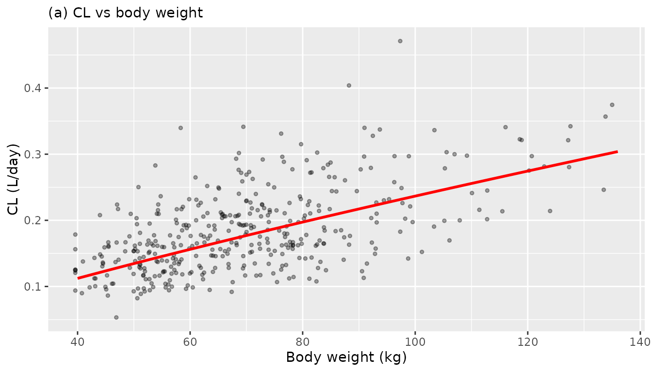
print(p_alb)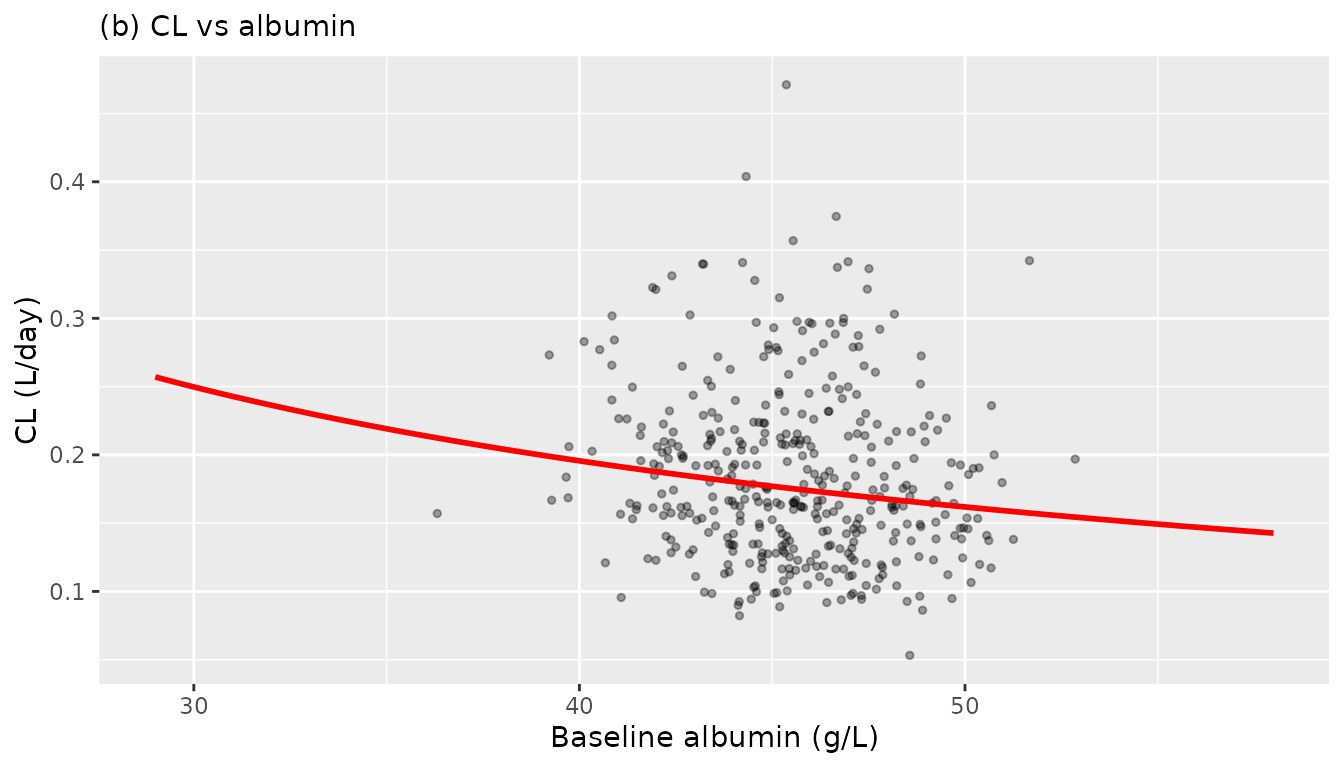
The red line is the typical-participant prediction at the other covariate’s reference value, matching the model-predicted line overlaid in Figure 3. CL rises with body weight and falls with albumin, the directions the paper reports.
Figure S1 – median profile of the approved regimen
# Replicates Figure S1 of Ait-Oudhia 2024: median (2.5th-97.5th percentile)
# profile under the FDA-approved regimen, 0.3 mg/kg followed by 0.7 mg/kg Q3W.
sim |>
  filter(cohort == "PAH 0.3 then 0.7 mg/kg Q3W", !is.na(Cc)) |>
  group_by(time) |>
  summarise(
    Q025 = quantile(Cc, 0.025, na.rm = TRUE),
    Q50  = quantile(Cc, 0.500, na.rm = TRUE),
    Q975 = quantile(Cc, 0.975, na.rm = TRUE),
    .groups = "drop"
  ) |>
  ggplot(aes(time, Q50)) +
  geom_ribbon(aes(ymin = Q025, ymax = Q975), alpha = 0.25) +
  geom_line(linewidth = 0.8) +
  labs(
    x = "Time (days)", y = "Sotatercept concentration (mg/L)",
    title = "Approved regimen: 0.3 mg/kg then 0.7 mg/kg Q3W",
    caption = "Replicates Figure S1 of Ait-Oudhia 2024 (median, 2.5th-97.5th percentiles)."
  )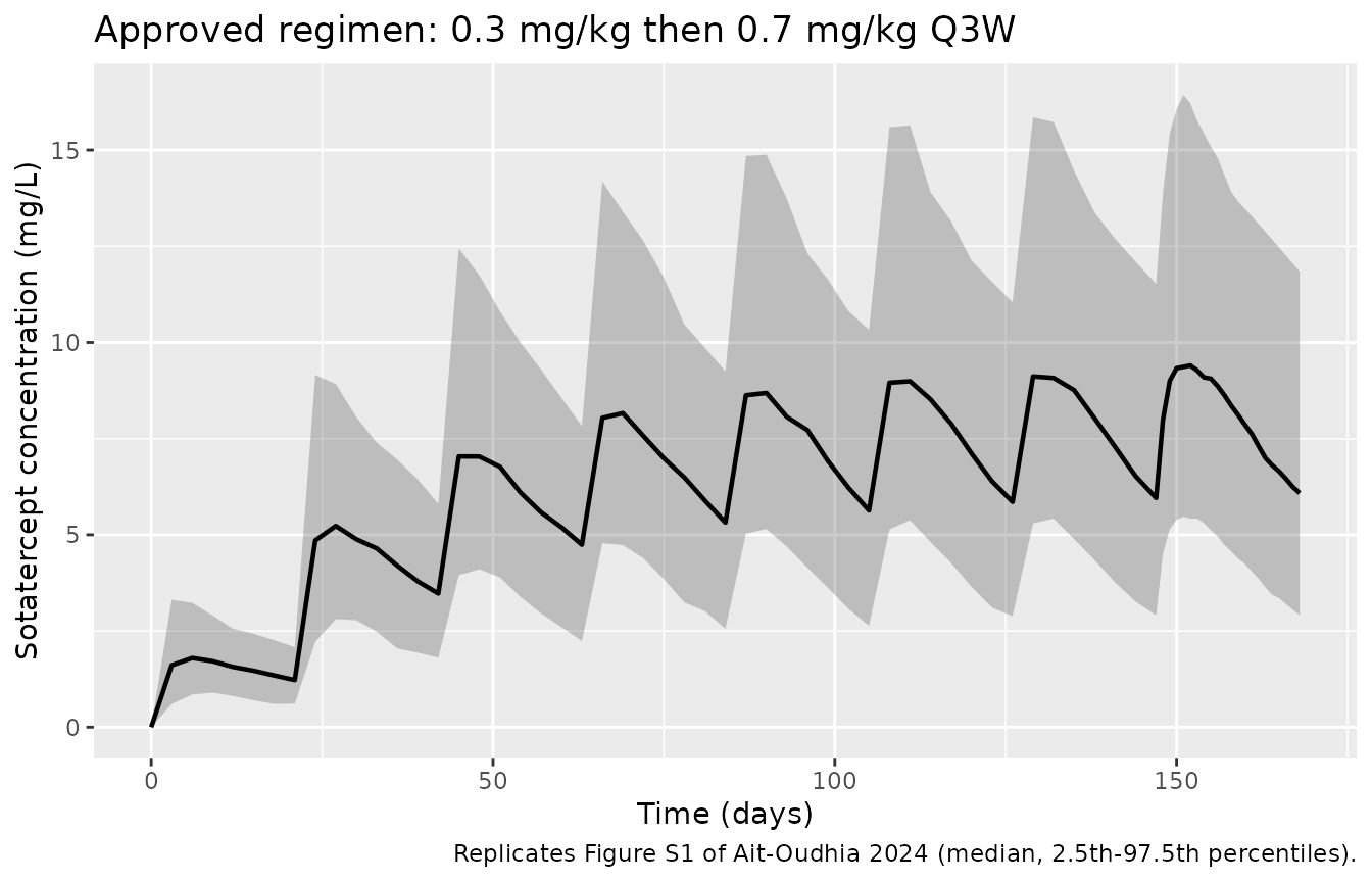
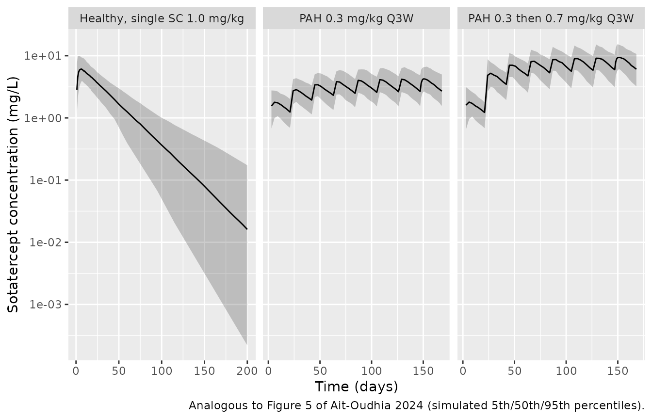
Figure 5 – prediction interval by cohort
# Analogous to Figure 5 of Ait-Oudhia 2024 (pcVPC stratified by study and
# route). Observed data are unavailable, so this shows the simulated
# 5th/50th/95th percentiles on a log y-axis.
sim |>
  filter(!is.na(Cc)) |>
  group_by(cohort, time) |>
  summarise(
    Q05 = quantile(Cc, 0.05, na.rm = TRUE),
    Q50 = quantile(Cc, 0.50, na.rm = TRUE),
    Q95 = quantile(Cc, 0.95, na.rm = TRUE),
    .groups = "drop"
  ) |>
  filter(Q05 > 0) |>
  ggplot(aes(time, Q50)) +
  geom_ribbon(aes(ymin = Q05, ymax = Q95), alpha = 0.25) +
  geom_line() +
  facet_wrap(~cohort, scales = "free_x") +
  scale_y_log10() +
  labs(
    x = "Time (days)", y = "Sotatercept concentration (mg/L)",
    caption = "Analogous to Figure 5 of Ait-Oudhia 2024 (simulated 5th/50th/95th percentiles)."
  )
PKNCA validation
Single-dose arm (healthy participants)
sim_sd <- sim |>
  filter(cohort == "Healthy, single SC 1.0 mg/kg", !is.na(Cc)) |>
  # Per subject, keep Cc >= 1e-6 * Cmax after the peak: below that the ODE integrator has no relative accuracy left.
  group_by(id) |>
  filter(time <= time[which.max(Cc)] | Cc >= 1e-6 * max(Cc)) |>
  ungroup() |>
  select(id, time, Cc, cohort)

# Guarantee a time-zero row per subject; pre-dose Cc = 0 for an extravascular
# dose. Without it PKNCA warns that the AUC range starts before the first
# measurement, once per subject.
sim_sd <- bind_rows(
  sim_sd,
  sim_sd |> distinct(id, cohort) |> mutate(time = 0, Cc = 0)
) |>
  distinct(id, cohort, time, .keep_all = TRUE) |>
  arrange(id, time)

dose_sd <- events |>
  filter(cohort == "Healthy, single SC 1.0 mg/kg", evid == 1) |>
  select(id, time, amt, cohort)

conc_sd <- PKNCA::PKNCAconc(sim_sd, Cc ~ time | cohort + id,
                            concu = "mg/L", timeu = "day")
dobj_sd <- PKNCA::PKNCAdose(dose_sd, amt ~ time | cohort + id, doseu = "mg")

int_sd <- data.frame(
  start = 0, end = Inf,
  cmax = TRUE, tmax = TRUE, aucinf.obs = TRUE, half.life = TRUE
)

res_sd <- PKNCA::pk.nca(PKNCA::PKNCAdata(conc_sd, dobj_sd, intervals = int_sd))
summary(res_sd)
#>  Interval Start Interval End                       cohort   N Cmax (mg/L)
#>               0          Inf Healthy, single SC 1.0 mg/kg 200 6.54 [28.3]
#>         Tmax (day) Half-life (day) AUCinf,obs (day*mg/L)
#>  6.00 [2.00, 23.0]     24.0 [9.04]            245 [29.0]
#>
#> Caption: Cmax, AUCinf,obs: geometric mean and geometric coefficient of variation; Tmax: median and range; Half-life: arithmetic mean and standard deviation; N: number of subjects
Steady-state arms (patients with PAH)
sim_ss <- sim |>
  filter(DIS_HEALTHY == 0, !is.na(Cc)) |>
  select(id, time, Cc, cohort)

dose_ss <- events |>
  filter(DIS_HEALTHY == 0, evid == 1) |>
  select(id, time, amt, cohort)

conc_ss <- PKNCA::PKNCAconc(sim_ss, Cc ~ time | cohort + id,
                            concu = "mg/L", timeu = "day")
dobj_ss <- PKNCA::PKNCAdose(dose_ss, amt ~ time | cohort + id, doseu = "mg")

# Final dose is at day 147; the steady-state interval is the 21 days after it.
int_ss <- data.frame(
  start = 147, end = 168,
  cmax = TRUE, tmax = TRUE, cmin = TRUE, auclast = TRUE, cav = TRUE
)

res_ss <- PKNCA::pk.nca(PKNCA::PKNCAdata(conc_ss, dobj_ss, intervals = int_ss))
summary(res_ss)
#>  Interval Start Interval End                     cohort   N AUClast (day*mg/L)
#>             147          168          PAH 0.3 mg/kg Q3W 200        75.3 [31.1]
#>             147          168 PAH 0.3 then 0.7 mg/kg Q3W 200         168 [32.2]
#>  Cmax (mg/L) Cmin (mg/L)        Tmax (day)  Cav (mg/L)
#>  4.27 [28.9] 2.73 [37.4] 5.00 [2.00, 8.00] 3.59 [31.1]
#>  9.64 [29.9] 5.97 [39.1] 5.00 [2.00, 9.00] 8.01 [32.2]
#>
#> Caption: AUClast, Cmax, Cmin, Cav: geometric mean and geometric coefficient of variation; Tmax: median and range; N: number of subjects
Gate 5 – between-subject variability in steady-state AUC
auc_cv <- as.data.frame(res_ss) |>
  filter(PPTESTCD == "auclast", start == 147) |>
  group_by(cohort) |>
  summarise(
    `AUCtau geometric mean` = round(exp(mean(log(PPORRES))), 1),
    `AUCtau %CV` = round(sd(PPORRES) / mean(PPORRES) * 100, 1),
    .groups = "drop"
  )

auc_cv |>
  knitr::kable(
    caption = paste(
      "Gate 5: model-predicted between-subject variability in steady-state",
      "AUC over one dosing interval. Ait-Oudhia 2024 reports 'an observed 35%",
      "variability in sotatercept AUC' (Discussion)."
    )
)| cohort | AUCtau geometric mean | AUCtau %CV |
|---|---|---|
| PAH 0.3 mg/kg Q3W | 75.3 | 30.6 |
| PAH 0.3 then 0.7 mg/kg Q3W | 168.1 | 31.6 |
The model-predicted between-subject %CV in steady-state AUC is close to the roughly 35% variability the paper reports as observed. The simulated value is expected to sit slightly below the observed figure, because the observed variability additionally absorbs residual error and between-study heterogeneity that the model attributes to separate terms.
Comparison against published values
Ait-Oudhia 2024 reports no NCA table. The only NCA-style quantity it publishes is the terminal elimination half-life of about 22 days for a typical 70 kg participant with a median normal baseline albumin of 4.5 g/dL, so the comparison below runs PKNCA on the typical-value profile rather than on the stochastic cohort.
ev_typ <- rxode2::et(amt = 0.7 * 70, cmt = "depot") |>
  rxode2::et(sort(unique(c(seq(0, 30, by = 0.5), seq(31, 400, by = 2)))),
             cmt = "central")

sim_typ <- solve_typical(ev_typ) |>
  mutate(id = 1L, cohort = "Typical 70 kg, albumin 4.5 g/dL")

conc_typ <- PKNCA::PKNCAconc(
  # Keep Cc >= 1e-6 * Cmax after the peak: below that the ODE integrator has no relative accuracy left.
  sim_typ |> filter(!is.na(Cc), time <= time[which.max(Cc)] | Cc >= 1e-6 * max(Cc, na.rm = TRUE)) |>
    select(id, time, Cc, cohort),
  Cc ~ time | cohort + id, concu = "mg/L", timeu = "day"
)
dobj_typ <- PKNCA::PKNCAdose(
  tibble(id = 1L, time = 0, amt = 0.7 * 70,
         cohort = "Typical 70 kg, albumin 4.5 g/dL"),
  amt ~ time | cohort + id, doseu = "mg"
)

res_typ <- PKNCA::pk.nca(PKNCA::PKNCAdata(
  conc_typ, dobj_typ,
  intervals = data.frame(start = 0, end = Inf, half.life = TRUE,
                         cmax = TRUE, tmax = TRUE, aucinf.obs = TRUE)
))

published <- tibble::tibble(
  cohort = "Typical 70 kg, albumin 4.5 g/dL",
  half.life = 22
)

cmp <- nlmixr2lib::ncaComparisonTable(
  simulated = res_typ,
  reference = published,
  by = "cohort",
  units = c(half.life = "day"),
  tolerance_pct = 20
)

knitr::kable(
  cmp,
  caption = paste(
    "Simulated vs published terminal half-life.",
    "* marks a difference from the reference above 20%."
  )
)| NCA parameter | cohort | Reference | Simulated | % diff |
|---|---|---|---|---|
| t½ (day) | Typical 70 kg, albumin 4.5 g/dL | 22 | 21.7 | -1.6% |
t_half <- as.data.frame(res_typ) |>
  filter(PPTESTCD == "half.life") |>
  pull(PPORRES)

# Independent closed-form check using the paper's own beta-phase formula
# (Methods): beta = 0.5 * [(k12 + k21 + kel) - sqrt((k12+k21+kel)^2 - 4*k21*kel)].
k12 <- 0.487 / 3.60
k21 <- 0.487 / 1.71
kel <- 0.177 / 3.60
beta <- 0.5 * ((k12 + k21 + kel) - sqrt((k12 + k21 + kel)^2 - 4 * k21 * kel))
t_half_closed <- log(2) / beta

tibble(
  Source = c("PKNCA half.life on the typical profile",
             "Closed form from the paper's beta-phase equation",
             "Ait-Oudhia 2024 Discussion"),
  `t-half (days)` = c(round(t_half, 2), round(t_half_closed, 2), 22)
) |>
knitr::kable(caption = "Gate 1: terminal half-life, three ways.")| Source | t-half (days) |
|---|---|
| PKNCA half.life on the typical profile | 21.66 |
| Closed form from the paper’s beta-phase equation | 21.64 |
| Ait-Oudhia 2024 Discussion | 22.00 |
The PKNCA terminal half-life on the typical profile agrees with the closed-form beta-phase half-life computed from the paper’s own equation, and both round to the roughly 22 days the Discussion reports. Because this quantity depends jointly on CL, VC, Q, and VP, it is the strongest single end-to-end check available for this model.
Assumptions and deviations
-
Albumin units and reference value. The canonical
covariate register stores
ALBin SI g/L, whereas Ait-Oudhia 2024 reports albumin in US-convention g/dL and writes the Table 2 footnote a reference as 4.5 g/dL. Because albumin enters only as a reference-normalised ratio, that ratio is scale-invariant:(ALB_gL / 45)is identically(ALB_gdL / 4.5). The model file therefore uses a 45 g/L reference and reproduces the published equation exactly, with no conversion line and no change to the fitted exponent. -
Body weight held constant per subject. The paper
uses the time-varying weight column (
WTKGT) on both CL and VC over a follow-up of up to about 150 weeks. This vignette assigns each virtual subject a single baseline weight and holds it constant, because no published weight-trajectory data exist to simulate from. The model file itself imposes no such restriction – supplying a time-varyingWTcolumn reproduces the paper’s parameterisation directly. - Covariate distributions are reconstructed, not observed. Body weight is drawn from a log-normal matched to the per-study mean and SD in Table 1 and truncated to the reported range; albumin from a truncated normal on the same basis. Table 1 reports means and SDs only, so the distributional families are assumptions. Correlation between weight and albumin is not reported and is therefore not simulated, even though the Discussion notes that “albumin correlates with BW”.
-
Race, sex, age, BMI, renal function, ADA status, and
background PAH therapy are not simulated. All were screened by
the paper and none was retained in the final model, so they have no
effect on the packaged model’s predictions. They are documented in the
model file’s
covariatesDataExcludedmetadata to preserve the provenance of the covariate screen. -
DIS_HEALTHYaffects only the residual error. Disease status entered during forward selection but was not retained during backward elimination (Discussion), so in the final model the healthy-versus-PAH contrast changes only which of the two log-scale residual SDs applies. It does not shift any structural or random-effect parameter. -
No IIV on Q. Table 2 reports “NE” (not estimated)
in the Q variability column, so no
etalqis included. This is a faithful encoding, not an omission. -
The IIV on F1 is logit-normal, not log-normal.
Table 2 footnote d states that F1 used a logit IIV model assuming a
normal distribution, whereas all other parameters used exponential
(log-normal) IIV. The footnote’s own arithmetic,
100 x (1 - 0.659) x 0.348 = 11.9, identifies the logit-scale omega as 0.348 directly; that is the value encoded, rather than a value back-transformed from the reported 11.9 %CV under a log-normal assumption. -
Residual error is a variance in Table 2 and an SD in the
model file. Table 2’s “Final parameter estimate” column holds
the residual variance (0.0570 healthy, 0.0357 PAH) and its
“Magnitude of variability” column the corresponding SD (0.239, 0.189).
sqrt(0.0570) = 0.2387andsqrt(0.0357) = 0.1889confirm which column is which; the model file encodes the SDs, as nlmixr2’slnorm()expects. - Supplementary material was not available. Supplementary Material S1 (per-study dosing regimens and sampling schemes) and Figures S1 and S2 are not deposited in the PubMed Central open-access record and could not be retrieved. Neither contains parameter values – every estimate used here is from Table 2 of the main text – so the gap does not affect the extraction. The dosing regimens simulated above are taken from the Methods and Discussion narrative instead, and the Figure S1 replication is therefore a reconstruction of the described regimen rather than a digitised overlay.
-
Albumin effect size stated in prose versus the printed
equation. The Discussion says typical CL is “predicted to
decline by 30% from minimum to maximum values of ALB concentrations in
the totality of all participants”. The Table 2 footnote a equation
applied across the full Table 1 albumin range (2.9 to 5.8 g/dL) gives
(5.8/2.9)^-0.849 = 0.555, a 44% decline. The 30% figure is consistent with a narrower interval (a ratio of about 1.52, e.g. 3.6 to 5.5 g/dL) and is most likely quoted over a percentile range rather than the observed extremes. Per the standing convention that the printed equation takes precedence over prose, the exponent -0.849 is encoded as published and no adjustment was made. - No erratum applies. A search of PubMed, the Wiley/ASCPT landing page, and the EuropePMC comment-and-correction list for doi:10.1002/psp4.13166 returned no erratum, corrigendum, or author correction as of the extraction date.
- A companion PK/PD paper exists and is out of scope here. Ait-Oudhia et al. published a follow-on population PK/PD and exposure-response analysis of sotatercept in 2025 (Clin Pharmacol Ther, doi:10.1002/cpt.3524). This vignette covers only the 2024 popPK paper; the PD and exposure-response layers are a separate extraction.