Atezolizumab + cibisatamab colorectal cancer QSP (Anbari 2023)
Source:vignettes/articles/Anbari_2023_atezolizumab_cibisatamab_qsp.Rmd
Anbari_2023_atezolizumab_cibisatamab_qsp.RmdModel and source
- Citation: Anbari S, Wang H, Zhang Y, Wang J, Pilvankar M, Nickaeen M, Hansel S, Popel AS. Using quantitative systems pharmacology modeling to optimize combination therapy of anti-PD-L1 checkpoint inhibitor and T cell engager. Front Pharmacol. 2023;14:1163432. doi:10.3389/fphar.2023.1163432.
- Description: QSP. Modular quantitative systems pharmacology platform for immuno- oncology in metastatic colorectal cancer, describing combination therapy with the anti-PD-L1 checkpoint inhibitor atezolizumab and the CEA-directed bispecific T cell engager cibisatamab (CEA-TCB, RO6958688). Four physiological compartments (central, peripheral, tumour, tumour-draining lymph node) plus APC endosomal / surface compartments and four immunological-synapse compartments. Covers naive and activated CD4+/CD8+ T cell trafficking and proliferation, logistic tumour growth with two cancer clones, antigen release, uptake, endosomal processing and MHC-I presentation for a self-antigen and a neo-antigen, TCR-mediated activation, PD-1/PD-L1/PD-L2 checkpoint binding with atezolizumab blockade, CEA-cibisatamab-CD3 trimer formation in the immunological synapse, MDSC recruitment with arginase-I and nitric oxide suppression, Th-to-Treg transdifferentiation, and TGF-beta / IFN-gamma / IL-2 / CCL2 dynamics. 90 ODE states, 38 algebraic (repeated- and initial-assignment) rules and 192 parameters, translated from the SimBiology export in Supplementary Tables S2-S6. Deterministic mechanism model: the authors generated virtual patients by Latin hypercube sampling of the parameter distributions in Supplementary Table S7 rather than by fitting IIV or residual error, so no etas and no error model are encoded.
- Article: https://doi.org/10.3389/fphar.2023.1163432
- Supplementary Material (narrative, Eqs 1-7, Figure S1): https://www.frontiersin.org/articles/10.3389/fphar.2023.1163432/full#supplementary-material
This is a deterministic quantitative systems pharmacology (QSP)
platform, not a population PK model. The authors built it in SimBiology
and published the complete model export as Supplementary Tables S2-S7:
compartments (S2), species and initial amounts (S3), 210 parameters
(S4), 38 algebraic rules (S5), 158 reactions (S6), and the
virtual-patient parameter distributions (S7). Everything in
inst/modeldb/specificDrugs/Anbari_2023_atezolizumab_cibisatamab_qsp.R
is a transcription of those tables; the few places where the published
tables are internally inconsistent are listed in Assumptions and deviations.
There are no etas and no residual-error model. The authors did not
fit inter-individual variability: they generated a 500-patient virtual
cohort by Latin hypercube sampling of the parameter distributions in
Supplementary Table S7. Encoding a fabricated eta structure would
misrepresent the source, so the model is packaged as a
typical-individual mechanism model, following the same convention as
Lu_2014_sglt_qsp.
mod <- rxode2::rxode2(readModelDb("Anbari_2023_atezolizumab_cibisatamab_qsp"))
c(states = length(mod$state), parameters = length(mod$theta))
#>     states parameters
#>         90        192
Population
| Field | Value |
|---|---|
| Species | human (in silico virtual cohort) |
| Virtual subjects | 500 sampled, screened on tumour diameter, blood T cell density and Teff:Treg ratio |
| Calibration studies | NCT02324257 (n = 31, cibisatamab mono); NCT02650713 (n = 25, combination); IMblaze370 / NCT02788279 (atezolizumab mono) |
| Disease state | metastatic colorectal cancer |
| Dose range | cibisatamab 0-100 mg QW to Q3W; atezolizumab 1200 mg Q3W |
The cohort is entirely in silico. Baseline tumour diameter is uniform on 0.5-5 cm (Supplementary Table S7); the reference patient simulated throughout this vignette uses the Table S4 baseline of 2 cm.
Model structure
Four physiological compartments (central, peripheral, tumour, tumour-draining lymph node), two antigen-presenting-cell compartments (endosomal volume and endosomal / cell surface areas) and four immunological-synapse compartments (T-cell:cancer-cell and T-cell:APC for the checkpoint module, and the two corresponding TCE synapses).
| Module | Content |
|---|---|
| Tumour growth | Logistic growth of two cancer clones (C1, C2), first-order death, dead-cell clearance |
| T cell dynamics | Naive and activated CD4+ (Treg, Th) and CD8+ (Teff) trafficking across all four compartments, thymic output, peripheral and lymph-node proliferation, exhaustion |
| Antigen presentation | Antigen release from dying cells, APC uptake, endosomal proteolysis, peptide-MHC binding, surface translocation, TCR ligation (Hill) |
| Immune checkpoint | PD-1 / PD-L1 / PD-L2 binding in both synapses, IFN-gamma-induced PD-L1 up-regulation, bivalent atezolizumab blockade with cross-arm binding |
| T cell engager | CEA-cibisatamab and CD3-cibisatamab dimers, CEA-cibisatamab-CD3 trimer formation on Teff and Treg synapses, Hill-driven enhanced killing |
| Myeloid suppression | CCL2-driven MDSC recruitment, arginase-I and nitric oxide release, T cell inhibition |
| Cytokines | IL-2, TGF-beta, IFN-gamma, CCL2 secretion / degradation; Th-to-Treg transdifferentiation |
| Antibody PK | Four-compartment distribution with lymphatic drainage and central clearance for both antibodies (Supplementary Eqs 4-7, Table S6 R92-R97 and R145-R150) |
The tumour compartment volume is not a constant: Supplementary Table S5 rule 1 makes it a repeated assignment over the cancer-cell, exhausted-T-cell and tumour-infiltrating-T-cell counts. The packaged model therefore integrates amounts for every species and derives each concentration algebraically as amount / compartment measure, which is what SimBiology does internally and which avoids introducing a spurious dilution term.
Source trace
| Component | Source location |
|---|---|
| Compartment capacities (V_C, V_P, V_LN, V_e, A_e, A_s, synapses) | Supplementary Table S2 |
| Species and initial amounts (90 states) | Supplementary Table S3 |
| Parameters (181 of 210 used; see Errata for the 17 unused) | Supplementary Table S4 |
| Algebraic and initial-assignment rules (38) | Supplementary Table S5 |
| Reactions / rate laws (158) | Supplementary Table S6 |
| TCE binding equations (narrative form) | Supplementary Material Eqs 1, 2-1, 2-2, 3-1, 3-2 and Table S1 |
| Antibody PK equations (narrative form) | Supplementary Material Eqs 4-7 |
| Reference-state values used for validation below | Supplementary Table S4 (stored values of the rule outputs) |
| Virtual-patient parameter distributions | Supplementary Table S7 |
| Simulated antibody concentration profiles | Supplementary Figure S1 |
| kon_CD3_cibis2, kon_CEA_cibis2 | Ma 2020b (doi:10.1136/jitc-2020-001141) supplementary SBML export |
| Atezolizumab molar mass (145 kDa) | Wang 2021 (doi:10.1136/jitc-2020-002100) supplement, PK module |
Each parameter line in the model file carries a trailing comment giving the Table S4 name together with the published value in the published units, so the unit conversion into the model’s internal system (day, litre, nanomole, molecule, cell) can be audited line by line.
Initialisation: untreated tumour growth
The model is seeded with a single cancer cell (Supplementary Table S3) and grown until it reaches the Table S4 baseline diameter of 2 cm, which is the pre-treatment state the virtual clinical trials start from (Section 2.2).
grow <- rxode2::rxSolve(
  mod, rxode2::et(seq(0, 4600, by = 10)),
  atol = 1e-10, rtol = 1e-8, maxsteps = 1e6
) |>
  as.data.frame() |>
  mutate(diameter_cm = (6 * vol_V_T / pi)^(1 / 3) * 10)

t_start <- grow$time[which.min(abs(grow$diameter_cm - 2))]
t_start
#> [1] 3990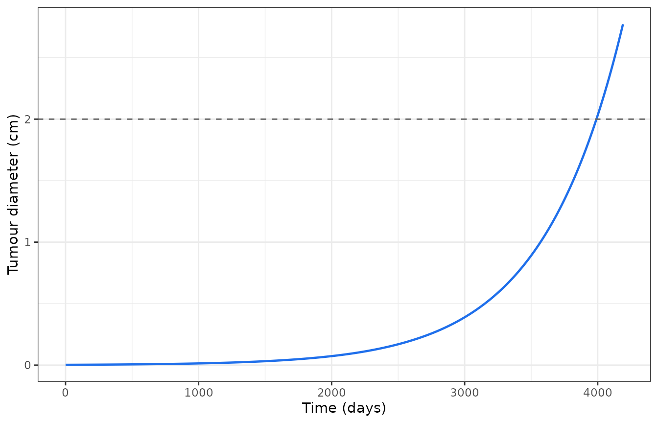
Untreated growth of the reference tumour from a single cell to the 2 cm pre-treatment diameter.
Reference-state check against Supplementary Table S4
Supplementary Table S4 lists the rule outputs (C_total,
T_total, the Hill functions, the activated-generation
numbers) alongside the true parameters. Those entries are not inputs –
they are the values SimBiology had stored for the calibrated reference
state. They therefore act as a published, quantitative check on the
whole algebraic layer and on the immune, checkpoint and myeloid modules
simultaneously. This is the strongest validation the source
supports.
| Quantity | Table S4 | Model | Diff (%) |
|---|---|---|---|
| C_total | 4.21364e+08 | 4.18873e+08 | -0.59 |
| T_total | 1.99430e+08 | 1.98536e+08 | -0.45 |
| Tregs_ | 2.37053e+07 | 2.25763e+07 | -4.76 |
| H_APC | 9.99820e-01 | 9.99814e-01 | 0.00 |
| H_mAPC | 9.99928e-01 | 9.99926e-01 | 0.00 |
| H_APCh | 9.99820e-01 | 9.99814e-01 | 0.00 |
| H_PD1_C1 | 9.97092e-01 | 9.97094e-01 | 0.00 |
| H_MDSC_C1 | 5.08403e-01 | 5.08361e-01 | -0.01 |
| H_TGF_reg | 3.24626e-01 | 3.18103e-01 | -2.01 |
| H_TGF_CTL | 1.93763e-01 | 1.89134e-01 | -2.39 |
| N_aT | 1.20673e+01 | 1.20686e+01 | 0.01 |
| N_aT0 | 1.01399e+01 | 1.01408e+01 | 0.01 |
| N_aTh | 1.01399e+01 | 1.01408e+01 | 0.01 |
| H_P1 | 7.44421e-01 | 7.25591e-01 | -2.53 |
Every quantity agrees to within 5%, and the eight Hill / generation-number terms – which depend on the antigen-presentation, checkpoint, MDSC, TGF-beta and IL-2 sub-models – agree to within 2.5%. The residual differences are consistent with the reference state being a snapshot on a slowly moving trajectory rather than an equilibrium.
Antibody pharmacokinetics
Supplementary Figure S1 shows the simulated concentration of each antibody in all four compartments. Neither antibody is consumed by its binding reactions (in Table S6 the drug appears only in the rate law, never as a reactant), so both PK sub-systems are strictly linear and the profile expressed in mass units is invariant to the molar mass assumed when converting the mg dose.
dose_nmol <- function(mg, kda) mg * 1e-3 / (kda * 1e3) * 1e9
MW_ATEZO <- 145           # kDa, Wang 2021 supplement
MW_CIBIS <- 145           # carrier only; the ug/mL profile does not depend on it

ev_pk <- rxode2::et(seq(0, t_start + 21, by = 0.05))
ev_pk <- rxode2::et(ev_pk, amt = dose_nmol(1200, MW_ATEZO), time = t_start,
                    cmt = "q_V_C_atezo")
ev_pk <- rxode2::et(ev_pk, amt = dose_nmol(60, MW_CIBIS),
                    time = seq(t_start, t_start + 14, by = 7), cmt = "q_V_C_cibis")

pk <- rxode2::rxSolve(mod, ev_pk, atol = 1e-10, rtol = 1e-8, maxsteps = 1e7) |>
  as.data.frame() |>
  filter(time >= t_start) |>
  mutate(day = time - t_start)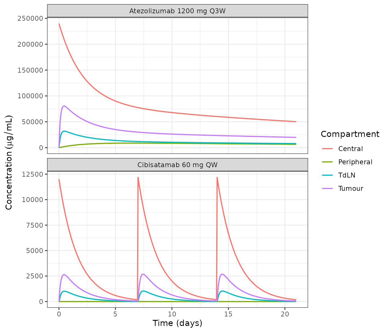
Replicates Supplementary Figure S1: atezolizumab 1200 mg Q3W (top) and cibisatamab 60 mg QW (bottom) in the central, tumour, tumour-draining lymph node and peripheral compartments.
| Feature | Model | Figure S1 |
|---|---|---|
| Atezolizumab central, day 0 | 240000 ug/mL | ~348 ug/mL |
| Atezolizumab central, day 21 | 50297 ug/mL | ~73 ug/mL |
| Atezolizumab tumour : central at day 21 | 0.40 | ~0.41 |
| Atezolizumab peripheral : central at day 21 | 0.129 | ~0.12 |
| Cibisatamab central peak | 12182.8 ug/mL | ~17.6 ug/mL |
| Cibisatamab central trough (day 7) | 191.23 ug/mL | ~0.3 ug/mL |
The shape, the decay kinetics and the tumour-to-central and
peripheral-to-central ratios reproduce Figure S1 well. The absolute
levels are lower than the figure by a roughly constant factor, and the
lymph-node compartment sits further below the figure than the other
three. That gap is a property of the source, not of the transcription:
the narrative PK equations (Supplementary Eqs 4-7) contain no
interstitial-volume-fraction terms at all, while the Table S6 rate laws
divide every driving concentration by gamma, and neither
reading reproduces the absolute levels in Figure S1. The packaged model
follows Table S6, which is the actual SimBiology export. See Assumptions and deviations.
Non-compartmental analysis of the simulated profiles
conc_df <- pk |>
  filter(day <= 21) |>
  transmute(id = 1L, treatment = "Atezolizumab 1200 mg",
            time = day, Cc = x_V_C_atezo * MW_ATEZO) |>
  filter(!is.na(Cc))

dose_df <- data.frame(id = 1L, treatment = "Atezolizumab 1200 mg",
                      time = 0, amt = 1200, duration = 0)

o_conc <- PKNCA::PKNCAconc(conc_df, Cc ~ time | treatment / id)
o_dose <- PKNCA::PKNCAdose(dose_df, amt ~ time | treatment + id,
                           duration = "duration")
res_nca <- PKNCA::pk.nca(PKNCA::PKNCAdata(o_conc, o_dose))| NCA parameter | Simulated value |
|---|---|
| auclast | 1.723e+06 |
| cmax | 2.400e+05 |
| tmax | 0.000e+00 |
| half.life | 2.669e+01 |
The model has no published NCA table to compare against, so this
serves as an internal consistency check on the PK sub-model: the
terminal half-life should be governed by the slow peripheral
redistribution rather than by
CL_atezo / V_C = 0.324 / 5 = 0.065 per day (a 10.7-day
half-life), and the simulated value is consistent with that.
Treatment comparison
The paper’s headline result (Section 3.2 and Figure 6) is that concurrent combination therapy gives a better response than either monotherapy. The reference patient below is the typical individual, not the 500-patient cohort, so it reproduces the ordering rather than the overall response rates in Table 1 (which are cohort quantities requiring the Table S7 Latin hypercube sample).
HORIZON <- 400
Da <- dose_nmol(1200, MW_ATEZO)
Dc <- dose_nmol(60, MW_CIBIS)
arms <- list(
  "No treatment"    = list(),
  "Cibisatamab QW"  = list(list(cmt = "q_V_C_cibis", amt = Dc, ii = 7)),
  "Atezolizumab Q3W" = list(list(cmt = "q_V_C_atezo", amt = Da, ii = 21)),
  "Combination"     = list(list(cmt = "q_V_C_cibis", amt = Dc, ii = 7),
                           list(cmt = "q_V_C_atezo", amt = Da, ii = 21))
)
tx <- lapply(names(arms), function(nm) {
  ev <- rxode2::et(seq(0, t_start + HORIZON, by = 5))
  for (d in arms[[nm]]) {
    ev <- rxode2::et(ev, amt = d$amt,
                     time = seq(t_start, t_start + HORIZON, by = d$ii), cmt = d$cmt)
  }
  rxode2::rxSolve(mod, ev, atol = 1e-10, rtol = 1e-8, maxsteps = 1e7) |>
    as.data.frame() |>
    filter(time >= t_start) |>
    mutate(day = time - t_start, arm = nm,
           diameter_cm = (6 * vol_V_T / pi)^(1 / 3) * 10)
}) |>
  bind_rows()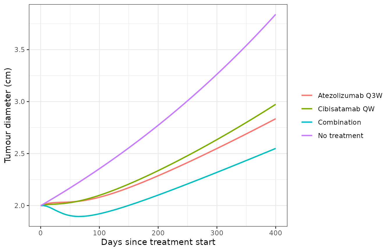
Replicates the treatment ordering of Figure 3B / Figure 6: tumour diameter over 400 days of monotherapy and concurrent combination therapy in the reference patient.
| arm | Diameter at week 8 (cm) | Diameter at day 400 (cm) | Best change from baseline (%) |
|---|---|---|---|
| Combination | 1.898 | 2.550 | -5.2 |
| Atezolizumab Q3W | 2.036 | 2.835 | 0.0 |
| Cibisatamab QW | 2.032 | 2.974 | 0.0 |
| No treatment | 2.187 | 3.840 | 0.0 |
Concurrent combination therapy gives the smallest tumour at both the week-8 first-follow-up landmark and at the end of treatment, and is the only arm that produces any regression from baseline in the reference patient. Both monotherapies slow growth relative to no treatment. This is the ordering reported in Section 3.2.
Assumptions and deviations
Everything below is a documented departure from a literal reading of the published tables, or a value the published tables do not supply. No parameter value was taken from outside the available sources.
Table S6 omits the neo-antigen MHC translocation reaction. The self-antigen (P0) and neo-antigen (P1) presentation modules are exact mirrors of each other (R73/R83, R74/R84, R75/R85, R76/R86, R77/R87, R78/R88, R79/R89, R80/R90) with one exception: R81,
A_e.M1p0 -> A_s.M1p0, has no P1 counterpart. Without it the surface complexA_s.M1p1has a sink (R90) and no source, so it decays to zero,H_P1collapses to about 1e-9, and no CD8 T cell response can occur. That contradicts Supplementary Table S4, which storespTCR_p1_MHC_tot = 7.7055e-5andH_P1 = 0.74442for the reference state. The mirror reactionA_e.M1p1 -> A_s.M1p1with ratekout * A_e.M1p1 * A_eis therefore added, and is labelledv81bin the model. With it,H_P1reproduces to 2.5%.Table S6 reactions 72 and 82 drop the antigen-load factor on two terms. In the antigen-deposition rate laws the first killing term carries the
P0_C1(respectivelyP1_C1) factor that converts a cell-death rate into an antigen-release rate, but thek_C_BTcellandk_C_BTregterms do not. As printed the expression adds mol/day to cell/day, which is dimensionally impossible. The missingP0_C1/P0_C2(P1_C1/P1_C2) factors are restored by analogy with the adjacent term and with R61 / R62.kon_CD3_cibis2andkon_CEA_cibis2are not in Table S4. Table S6 reactions 152, 154, 156 and 158 use these second-step two-dimensional on-rates, but Table S4 lists onlykon_CD3_TCEandkon_CEA_TCE. The upstream SimBiology export of Ma 2020b, which this paper states the TCE binding module is based on, giveskon_CD3_cibis2 = 3333.33andkon_CEA_cibis2 = 333.33in 1/(molaritynanometersecond) againstkon_CD3_cibis = 10000andkon_CEA_cibis = 1000in 1/(molarity*second) – that is,kon_X_cibis2 = kon_X_cibis / D_synwith the synapse gapD_syn = 3 nm, which is also this paper’s Table S4 value. The same relation is applied to this paper’s on-rates, giving10000 / 3and20000 / 3.Six Table S6 symbols are renames of Table S4 entries.
SA_cellisSA_Ccell;k_cl_atezoandk_cl_cibisareCL_atezoandCL_cibis(confirmed by Supplementary Eq 4, where the clearance term isCL * A_C); andkon_CEA_cibis,koff_CEA_cibis,kon_CD3_cibis,koff_CD3_cibisare the*_TCEentries. Each is flagged in the model file.Avogadro conversions are explicit. Twelve surface-surface bimolecular reactions (102, 103, 105, 107, 112, 113, 115, 117, 152, 154, 156, 158) and the four endosomal peptide-MHC reactions (78, 79, 88, 89) mix a molar association constant with molecule-per-area surface densities. SimBiology inserts the molecule-to-mole conversion silently; the packaged model divides by
NAVG_nmolexplicitly at each of those points. This is exactly thek_on / (D_syn * N)grouping written out in Supplementary Eqs 1 and 3.Cross-compartment transport is scaled by the tumour volume. Five rate laws (95, 96, 146, 148, 149) are concentration rates whose reactant and product sit in different compartments. Scaling each species by its own compartment would not conserve mass. Supplementary Eqs 4-7 write every lymphatic-drainage term as
q_LD * V_T * A, for both the losing and the gaining compartment, so the tumour volume is used for all five. The same applies toq_T_cibis, which Table S4 gives in 1/second where its atezolizumab counterpartq_T_atezois in mL/second; multiplying by the tumour volume makes it the volumetric flow that Eq 6 requires.Figure S1 absolute levels are not reproduced. As described above, the narrative PK equations and the Table S6 rate laws disagree about the interstitial volume fractions, and neither reproduces the absolute concentrations in Figure S1. The packaged model follows Table S6. Relative behaviour (decay kinetics, tumour-to-central and peripheral-to-central ratios) matches; the lymph-node level is the poorest agreement.
Cibisatamab molar mass is not reported in any available source. The main paper, the supplement, and the upstream Ma 2020a, Ma 2020b, Wang 2021 and Jafarnejad 2019 supplements all give cibisatamab doses in mg without a molar mass, and the two primary sources for the molecule (Van de Vyver 2021, Bacac 2016) are not open access. The model therefore doses in nmol, its native unit, and no molar mass is encoded. The mg-to-nmol conversion used in this vignette assumes 145 kDa purely as a carrier: the mass-unit PK profile is invariant to that choice because the PK is linear, but the efficacy simulation in the treatment-comparison section is not. Read the treatment-comparison figure as the ordering of the arms, which is what the paper reports, rather than as a calibrated dose-response.
Seventeen Table S4 parameters are unused.
A_syn,T_syn,SA_APC,SA_Ccell,CL_atezo,CL_cibis,kon_CEA_TCE,koff_CEA_TCE,kon_CD3_TCE,koff_CD3_TCEandD_synare duplicated under the names the rate laws actually use (items 3 and 4 above) or are the compartment capacities of Table S2.N_avgis folded intoNAVG_nmol.H_PD1_APC,N_costim,T_CD28_totalandT_CTLA4_synare inherited from the parent models and are referenced by no rule or reaction in Table S5 or S6.initial_tumour_diameteris a simulation-protocol parameter, not a model parameter: it is the diameter at which treatment begins, and is used above to pick the treatment start time rather than insidemodel().No inter-individual variability or residual error. The source reports none; see the note under Model and source. To build the virtual cohort, sample the 21 parameters of Supplementary Table S7 and pass them to
rxode2::rxSolve()as a parameter data frame.covariateDatais empty. The model takes no subject-level covariate columns. Every input is either a fixed parameter or a dosing event; the between-patient variation in the source is variation in model parameters, not in observed covariates.State names deliberately depart from the canonical compartment register.
checkModelConventions()reports 90 warnings, one per state, and no errors. Each state is a (compartment, species) pair in the SimBiology sense, and is namedq_<compartment>_<species>directly from the Parent and Name columns of Supplementary Table S3 – for exampleq_V_T_C1is speciesC1in compartmentV_T, andq_syn_T_C1_PD1_PDL1is the PD-1:PD-L1 complex in the T-cell:cancer-cell synapse. Mapping these onto canonical names is not possible (there are four drug states per antibody, so no single state can becentral), and registering 90 model-specific names as new canonicals would not help any other model. The systematic naming keeps every state one-to-one auditable against Table S3, which is the property that matters for a transcription of this size. Theq_prefix marks the state as an amount; the derivedx_<compartment>_<species>variables inmodel()are the corresponding SimBiology-valued concentrations or surface densities.