Topiramate (Lee 2024)

Model and source

• Citation: Lee S, Kim HC, Jang Y, Lee HS, Ahn SJ, Lee ST, Jung KH, Park KI, Jung KY, Oh J, Lee S, Yu KS, Jang IJ, Lee S, Chu K, Lee SK. Topiramate dosage optimization for effective antiseizure management via population pharmacokinetic modeling. Ann Clin Transl Neurol. 2024;11(2):424-435. doi:10.1002/acn3.51962. Structural model carried from Bae EK, Lee J, Shin JW, et al. Factors influencing topiramate clearance in adult patients with epilepsy: a population pharmacokinetic analysis. Seizure. 2016;37:8-12; all parameters re-estimated on the Lee 2024 dataset (Lee 2024 Table S1).
• Description: One-compartment population PK model with first-order absorption and elimination for topiramate (TPM) in Korean adults with epilepsy undergoing routine therapeutic drug monitoring (Lee 2024). Apparent clearance CL/F carries an additive enzyme-inducing antiseizure-medication term (separate coefficients in L/h for phenytoin, carbamazepine, oxcarbazepine and phenobarbital), a power effect of creatinine clearance normalized to 90 mL/min, and a power effect of the topiramate daily dose normalized to 100 mg/day; apparent volume Vd/F scales allometrically with body weight (exponent fixed at 1) centred at 62 kg. Absorption rate constant fixed at 2 /h. Inter-individual variability on CL/F only (31.0 %CV) with a proportional residual error of 27.8%. The structural model was carried from Bae 2016 and all parameters were re-estimated on the present therapeutic-drug-monitoring dataset.
• Article: https://doi.org/10.1002/acn3.51962
• Supplement (Table S1, final parameter estimates and bootstrap): https://doi.org/10.1002/acn3.51962 (Supporting Information file ACN3-11-424-s001.docx)

Lee 2024 is primarily a therapeutic-drug-monitoring (TDM) paper: its clinical question is what serum topiramate concentration is needed for an antiseizure response, and what concentration starts to produce ataxia. The population PK model is the instrument used to convert single spot serum measurements into steady-state exposure metrics (Cmax, Cmin, AUC24h) that the response and adverse-event analyses are then run against. That makes the PK model the load-bearing component of every conclusion in the paper, and it is the part extracted here.

Population

The model was estimated on 555 serum topiramate samples from 389 Korean adults with epilepsy, collected during routine outpatient care at Seoul National University Hospital between January 2017 and January 2022 (Lee 2024 Table 1). Mean age was 46.4 +/- 10.9 years and 50.5% of samples came from male patients. Mean body weight was 64.6 +/- 17.7 kg, but weight was documented for only 237 of the 555 samples (Lee 2024 Table 1 footnote a).

Fifty-three patients (76 samples) were on topiramate monotherapy; 340 patients (479 samples) were on antiseizure-medication polytherapy with a median of 3 [2-4] medications. Enzyme-inducing antiseizure medications (EIASMs) – carbamazepine, oxcarbazepine, phenytoin or phenobarbital – were co-prescribed for 55.3% of samples. The mean total daily topiramate dose was 178.4 +/- 117.9 mg/day and the mean spot serum level was 3.9 +/- 2.8 mg/L.

Regimens were stable for at least one month before sampling so steady state could be assumed, and the interval between sampling and the last dose was recorded for every sample. Inpatient measurements were excluded because of confounding acute illness. Serum topiramate was assayed by UPLC-MS/MS over a 0.25-50 mg/L calibration range; values below the 0.25 mg/L limit of quantification were discarded (M1 method).

The same information is available programmatically via readModelDb("Lee_2024_topiramate")()$population.

str(readModelDb("Lee_2024_topiramate")()$population)
#> List of 12
#>  $ species       : chr "human"
#>  $ n_subjects    : int 389
#>  $ n_studies     : int 1
#>  $ n_observations: int 555
#>  $ age_mean      : chr "46.4 +/- 10.9 years"
#>  $ weight_mean   : chr "64.6 +/- 17.7 kg (documented for 237 of 555 samples)"
#>  $ sex_female_pct: num 49.5
#>  $ race_ethnicity: Named num 100
#>   ..- attr(*, "names")= chr "Korean"
#>  $ disease_state : chr "Adults with epilepsy on chronic topiramate therapy (53 patients on topiramate monotherapy, 340 on antiseizure-m"| __truncated__
#>  $ dose_range    : chr "Mean total daily dose 178.4 +/- 117.9 mg/day (121.4 +/- 59.4 mg/day monotherapy; 187.5 +/- 122.3 mg/day polythe"| __truncated__
#>  $ regions       : chr "South Korea (Seoul National University Hospital)"
#>  $ notes         : chr "Retrospective therapeutic-drug-monitoring cohort sampled between January 2017 and January 2022 (Lee 2024 Table "| __truncated__

Source trace

Every ini() entry in inst/modeldb/specificDrugs/Lee_2024_topiramate.R carries an in-file comment naming its source location. They are collected here for review. All final parameter estimates come from Lee 2024 Table S1 (supplement), which reports both the estimation result with %RSE and a 1000-sample bootstrap median with 95% CI; the CL/F covariate equation is also printed in the Results text.

Equation / parameter	Value	Source location
CL/F = (theta1 + theta4*CBZ + theta5*OXC + theta6*PHT + theta7*PB) * (CLcr/90)^theta8 * (DOSE/100)^theta9	n/a	Table S1 structure block; also printed in Results (“Topiramate pharmacokinetics”)
Vd/F = theta2 * (WT/62)	n/a	Table S1 structure block; exponent stated in Results as “the exponent of 1”
lcl (theta1, CL/F intercept)	1.45 L/h (2.80% RSE)	Table S1 theta1; bootstrap 1.45 (1.37-1.54)
lvc (theta2, Vd/F at 62 kg)	78.1 L (22.0% RSE)	Table S1 theta2; bootstrap 76.6 (52.3-139)
lka (Ka)	2 /h, fixed	Table S1 row “Ka … Fixed at 2”
e_pht_cl (theta6)	1.02 L/h (24.8% RSE)	Table S1 theta6; bootstrap 1.04 (0.530-1.51)
e_cbz_cl (theta4)	0.703 L/h (15.4% RSE)	Table S1 theta4; bootstrap 0.701 (0.494-0.908)
e_oxc_cl (theta5)	0.419 L/h (21.9% RSE)	Table S1 theta5; bootstrap 0.419 (0.237-0.595)
e_pb_cl (theta7)	0.376 L/h (34.8% RSE)	Table S1 theta7; bootstrap 0.382 (0.149-0.652)
e_crcl_cl (theta8)	0.277 (42.6% RSE)	Table S1 theta8; bootstrap 0.279 (0.0501-0.515)
e_dose_tpm_cl (theta9)	0.193 (16.7% RSE)	Table S1 theta9; bootstrap 0.193 (0.129-0.258)
e_wt_vc (allometric exponent on Vd/F)	1, fixed	Table S1 Vd/F equation; Results “allometric scaling was applied with the exponent of 1”
etalcl (IIV on CL/F)	31.0 %CV (14.1% RSE) -> omega^2 = log(1 + 0.310^2) = 0.0917584	Table S1 omega CL/F; bootstrap 30.4 (18.9-38.8)
propSd (proportional residual error)	27.8% (6.20% RSE) -> 0.278	Table S1 sigma prop; bootstrap 27.7 (24.0-31.0)
d/dt(depot), d/dt(central) (one compartment, first-order absorption and elimination)	n/a	Results “the previously structured one-compartment model with first-order absorption and elimination” (structure carried from Bae 2016)

The printed CL/F equation is self-validating

Lee 2024 reports the comedication effects twice: as absolute coefficients in Table S1 / the Results equation, and as percentage increases in the Discussion (“topiramate CL/F increased by 70%, 48%, 29%, and 26% in patients co-administered with PHT, CBZ, OXC, and PB”). Because the comedication terms enter additively in L/h on the 1.45 L/h monotherapy intercept, each percentage must equal coefficient / 1.45. That is an independent check on the transcription of all five structural clearance parameters at once, and it is exact:

intercept <- 1.45
coefs <- c(PHT = 1.02, CBZ = 0.703, OXC = 0.419, PB = 0.376)
reported_pct <- c(PHT = 70, CBZ = 48, OXC = 29, PB = 26)

selfcheck <- tibble(
  Comedication = names(coefs),
  `Coefficient (L/h)` = as.numeric(coefs),
  `Implied % increase` = round(100 * coefs / intercept),
  `Reported % increase (Discussion)` = as.numeric(reported_pct)
)

# All four must agree exactly; this is a transcription gate on Table S1.
stopifnot(identical(
  as.numeric(selfcheck$`Implied % increase`),
  as.numeric(selfcheck$`Reported % increase (Discussion)`)
))

knitr::kable(
  selfcheck,
  caption = paste(
    "Table S1 clearance coefficients reproduce the percentage increases",
    "reported independently in the Lee 2024 Discussion, confirming both the",
    "additive functional form and the transcribed values."
  )
)

Table S1 clearance coefficients reproduce the percentage increases reported independently in the Lee 2024 Discussion, confirming both the additive functional form and the transcribed values.

Comedication	Coefficient (L/h)	Implied % increase	Reported % increase (Discussion)
PHT	1.020	70	70
CBZ	0.703	48	48
OXC	0.419	29	29
PB	0.376	26	26

Structural identity gates

Before any cohort simulation, three deterministic identities are checked directly against the published equations. These use no between-subject variability (omega = NA), so each is an exact algebraic statement about the packaged model rather than a statistical comparison.

mod <- readModelDb("Lee_2024_topiramate")

# Reference subject: the normalization point of every covariate term --
# WT 62 kg, CLcr 90 mL/min, 100 mg/day. At this point all three covariate
# multipliers collapse to 1, so CL/F must equal the bare intercept sum and
# Vd/F must equal theta2 exactly.
scenarios <- tibble(
  scenario   = c("Monotherapy", "+ Phenytoin", "+ Carbamazepine",
                 "+ Oxcarbazepine", "+ Phenobarbital"),
  CONMED_PHT = c(0, 1, 0, 0, 0),
  CONMED_CBZ = c(0, 0, 1, 0, 0),
  CONMED_OXC = c(0, 0, 0, 1, 0),
  CONMED_PB  = c(0, 0, 0, 0, 1)
) |>
  mutate(id = row_number(), WT = 62, CRCL = 90, DOSE_TPM_MGD = 100)

gate_ev <- bind_rows(
  scenarios |> mutate(time = 0, evid = 1L, amt = 50, ii = 12, ss = 1L,
                      cmt = "depot"),
  scenarios |> mutate(time = 1, evid = 0L, amt = NA_real_, ii = 0, ss = 0L,
                      cmt = "central")
) |>
  arrange(id, time, desc(evid))

gate <- rxode2::rxSolve(mod, gate_ev, omega = NA, keep = "scenario",
                        returnType = "data.frame") |>
  filter(!is.na(Cc)) |>
  select(scenario, cl, vc)
#> ℹ parameter labels from comments will be replaced by 'label()'
#> Warning: multi-subject simulation without without 'omega'

# Gate 1 -- CL/F at the reference point equals the intercept plus the
# comedication increment, in absolute L/h (Lee 2024 Table S1).
expected_cl <- c(1.45, 1.45 + 1.02, 1.45 + 0.703, 1.45 + 0.419, 1.45 + 0.376)
stopifnot(all(abs(gate$cl - expected_cl) < 1e-8))

# Gate 2 -- Vd/F at the 62 kg reference weight equals theta2 = 78.1 L exactly,
# for every scenario (comedication acts on CL/F only).
stopifnot(all(abs(gate$vc - 78.1) < 1e-8))

# Gate 3 -- the covariate multipliers are exactly 1 at the normalization point,
# i.e. (90/90)^0.277 * (100/100)^0.193 == 1.
stopifnot(abs(gate$cl[gate$scenario == "Monotherapy"] - 1.45) < 1e-12)

gate |>
  mutate(`Expected CL/F (L/h)` = expected_cl) |>
  rename("Scenario" = scenario, "Model CL/F (L/h)" = cl,
         "Model Vd/F (L)" = vc) |>
  knitr::kable(
    digits = 4,
    caption = paste(
      "Structural identity gates at the covariate normalization point",
      "(WT 62 kg, CLcr 90 mL/min, 100 mg/day). Model output matches the",
      "Lee 2024 Table S1 coefficients to machine precision."
    )
  )

Structural identity gates at the covariate normalization point (WT 62 kg, CLcr 90 mL/min, 100 mg/day). Model output matches the Lee 2024 Table S1 coefficients to machine precision.

Scenario	Model CL/F (L/h)	Model Vd/F (L)	Expected CL/F (L/h)
Monotherapy	1.450	78.1	1.450
+ Phenytoin	2.470	78.1	2.470
+ Carbamazepine	2.153	78.1	2.153
+ Oxcarbazepine	1.869	78.1	1.869
+ Phenobarbital	1.826	78.1	1.826

Dosing frequency is not reported: QD and BID bracket the published exposures

Lee 2024 reports total daily dose and never states the dosing frequency. This matters for Cmax and Cmin but not for AUC24h, which for linear PK equals daily dose / (CL/F) regardless of how the daily dose is split. That asymmetry gives a clean way to handle the gap: AUC24h becomes a strict frequency-independent gate, and Cmax / Cmin are bracketed between once-daily and twice-daily administration.

The bracket is built on the two strata that require no assumption about which enzyme-inducing medication a patient received: topiramate monotherapy, and polytherapy without an EIASM. For both, Table 1 supplies the mean daily dose and body weight, and the comedication indicators are all zero, so the typical-value profile is fully determined by published numbers.

# Typical-value steady-state profile. Steady state is imposed with ss = 1
# rather than by dosing from zero, because the terminal half-life (~35 h in the
# monotherapy stratum) is long relative to the dosing interval.
typ_profile <- function(daily_dose, tau, wt, comeds = c(0, 0, 0, 0)) {
  subj <- tibble(
    id = 1L, WT = wt, CRCL = 90, DOSE_TPM_MGD = daily_dose,
    CONMED_PHT = comeds[1], CONMED_CBZ = comeds[2],
    CONMED_OXC = comeds[3], CONMED_PB = comeds[4]
  )
  ev <- bind_rows(
    subj |> mutate(time = 0, evid = 1L, amt = daily_dose / (24 / tau),
                   ii = tau, ss = 1L, cmt = "depot"),
    subj |> tidyr::crossing(time = seq(0, tau, by = 0.02)) |>
      mutate(evid = 0L, amt = NA_real_, ii = 0, ss = 0L, cmt = "central")
  ) |>
    arrange(id, time, desc(evid))
  rxode2::rxSolve(mod, ev, omega = NA, returnType = "data.frame") |>
    filter(!is.na(Cc))
}

# The two inducer-free strata of Table 1, with their published comparators.
bracket_strata <- tibble::tribble(
  ~stratum,                     ~daily_dose, ~wt,  ~pub_cmax, ~pub_cmin, ~pub_auc, ~pub_cl,
  "Monotherapy",                      121.4, 59.8,       4.0,       3.0,     84.4,     1.5,
  "Polytherapy without EIASM",        176.5, 65.2,       5.1,       3.8,    107.0,     1.6
)

bracket <- bind_rows(lapply(seq_len(nrow(bracket_strata)), function(i) {
  s <- bracket_strata[i, ]
  bind_rows(
    typ_profile(s$daily_dose, 24, s$wt) |> mutate(Regimen = "Once daily (24 h)"),
    typ_profile(s$daily_dose, 12, s$wt) |> mutate(Regimen = "Twice daily (12 h)")
  ) |>
    mutate(stratum = s$stratum, daily_dose = s$daily_dose)
}))

bracket_tab <- bracket |>
  group_by(stratum, Regimen) |>
  summarise(
    Cmax = max(Cc), Cmin = min(Cc),
    ratio = max(Cc) / min(Cc),
    AUC24h = first(daily_dose) / first(cl),
    CL = first(cl),
    .groups = "drop"
  )

# Gate 1 -- AUC24h is frequency-independent (it equals daily dose / CL/F), so
# the QD and BID values must be identical and must match the published AUC24h.
auc_check <- bracket_tab |>
  group_by(stratum) |>
  summarise(spread = diff(range(AUC24h)), auc = first(AUC24h), .groups = "drop") |>
  left_join(bracket_strata |> select(stratum, pub_auc), by = "stratum")
stopifnot(all(auc_check$spread < 1e-8))
stopifnot(all(abs(auc_check$auc / auc_check$pub_auc - 1) < 0.10))

# Gate 2 -- CL/F reproduces the published stratum value (no inducers involved,
# so this is an exact test of the intercept and the dose power term).
cl_check <- bracket_tab |>
  distinct(stratum, CL) |>
  left_join(bracket_strata |> select(stratum, pub_cl), by = "stratum")
stopifnot(all(abs(cl_check$CL / cl_check$pub_cl - 1) < 0.05))

# Gate 3 -- the published Cmax, Cmin and peak-to-trough ratio must each fall
# between the QD and BID profiles. Compared at the paper's own reported
# precision (one decimal place for concentrations), since the published values
# are rounded.
bracket_gate <- bracket_tab |>
  group_by(stratum) |>
  summarise(
    cmax_lo = round(min(Cmax), 1), cmax_hi = round(max(Cmax), 1),
    cmin_lo = round(min(Cmin), 1), cmin_hi = round(max(Cmin), 1),
    ratio_lo = min(ratio),         ratio_hi = max(ratio),
    .groups = "drop"
  ) |>
  left_join(bracket_strata, by = "stratum")

stopifnot(
  all(bracket_gate$pub_cmax >= bracket_gate$cmax_lo),
  all(bracket_gate$pub_cmax <= bracket_gate$cmax_hi),
  all(bracket_gate$pub_cmin >= bracket_gate$cmin_lo),
  all(bracket_gate$pub_cmin <= bracket_gate$cmin_hi),
  all(bracket_gate$pub_cmax / bracket_gate$pub_cmin >= bracket_gate$ratio_lo),
  all(bracket_gate$pub_cmax / bracket_gate$pub_cmin <= bracket_gate$ratio_hi)
)

bracket_tab |>
  select(-CL) |>
  bind_rows(
    bracket_strata |>
      transmute(stratum, Regimen = "Lee 2024 Table 1",
                Cmax = pub_cmax, Cmin = pub_cmin,
                ratio = pub_cmax / pub_cmin, AUC24h = pub_auc)
  ) |>
  arrange(stratum, Regimen) |>
  rename("Stratum" = stratum, "Cmax (mg/L)" = Cmax, "Cmin (mg/L)" = Cmin,
         "Cmax/Cmin" = ratio, "AUC24h (h*mg/L)" = AUC24h) |>
  knitr::kable(
    digits = 2,
    caption = paste(
      "Typical-value steady-state exposure for the two inducer-free strata.",
      "In both, the published Cmax, Cmin and peak-to-trough ratio fall between",
      "the once-daily and twice-daily profiles, and the frequency-independent",
      "AUC24h matches within 5%."
    )
  )

Typical-value steady-state exposure for the two inducer-free strata. In both, the published Cmax, Cmin and peak-to-trough ratio fall between the once-daily and twice-daily profiles, and the frequency-independent AUC24h matches within 5%.

Stratum	Regimen	Cmax (mg/L)	Cmin (mg/L)	Cmax/Cmin	AUC24h (h*mg/L)
Monotherapy	Lee 2024 Table 1	4.00	3.00	1.33	84.40
Monotherapy	Once daily (24 h)	4.08	2.65	1.54	80.65
Monotherapy	Twice daily (12 h)	3.66	3.00	1.22	80.65
Polytherapy without EIASM	Lee 2024 Table 1	5.10	3.80	1.34	107.00
Polytherapy without EIASM	Once daily (24 h)	5.50	3.59	1.53	109.08
Polytherapy without EIASM	Twice daily (12 h)	4.95	4.07	1.22	109.08

pub_lines <- bracket_strata |>
  select(stratum, pub_cmax, pub_cmin) |>
  tidyr::pivot_longer(c(pub_cmax, pub_cmin), values_to = "y")

ggplot(bracket, aes(time, Cc, colour = Regimen)) +
  geom_line(linewidth = 0.9) +
  geom_hline(data = pub_lines, aes(yintercept = y), linetype = "dashed",
             colour = "grey35") +
  facet_wrap(~stratum) +
  labs(x = "Time since dose (h)", y = "Serum topiramate (mg/L)",
       colour = NULL,
       title = "Steady-state profiles bracket the published Cmax and Cmin",
       caption = paste(
         "Dashed lines are the Lee 2024 Table 1 Cmax and Cmin for each",
         "stratum."
       )) +
  theme_bw() +
  theme(legend.position = "bottom")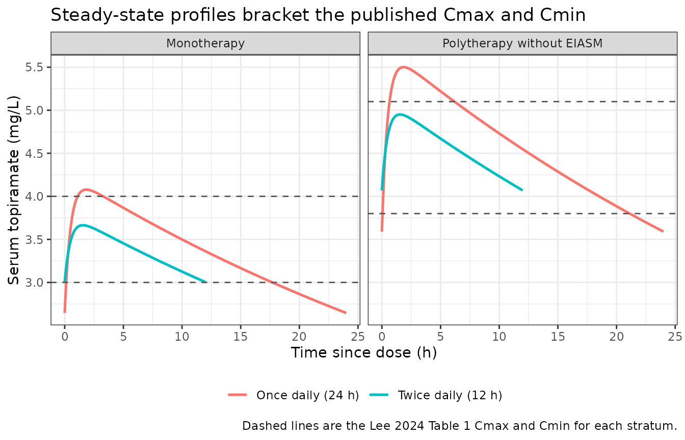

Typical-value steady-state topiramate profiles for the two inducer-free strata under once-daily and twice-daily administration. Dashed lines mark the Cmax and Cmin reported in Lee 2024 Table 1 for that stratum; both fall between the two regimens.

The remainder of the vignette uses twice-daily dosing, the labelled adult epilepsy regimen for topiramate.

The EIASM stratum is bracketed by the identity of the inducer

For the third stratum Lee 2024 reports that an EIASM was on board but not which one, and the four coefficients span a 2.7-fold range (0.376 to 1.02 L/h). Rather than assume a mix for this gate, the four inducers are each run alone at that stratum’s mean daily dose; the published CL/F and AUC24h must fall inside the resulting range.

inducers <- tibble::tribble(
  ~Inducer,          ~pht, ~cbz, ~oxc, ~pb,
  "Phenytoin",          1,    0,    0,   0,
  "Carbamazepine",      0,    1,    0,   0,
  "Oxcarbazepine",      0,    0,    1,   0,
  "Phenobarbital",      0,    0,    0,   1
)

eiasm <- bind_rows(lapply(seq_len(nrow(inducers)), function(i) {
  p <- typ_profile(193.6, 12, 65.2,
                   comeds = as.numeric(inducers[i, c("pht", "cbz", "oxc", "pb")]))
  tibble(
    Inducer = inducers$Inducer[i],
    `CL/F (L/h)` = p$cl[1],
    `Cmax (mg/L)` = max(p$Cc),
    `Cmin (mg/L)` = min(p$Cc),
    `AUC24h (h*mg/L)` = 193.6 / p$cl[1]
  )
}))

# Published EIASM-stratum values (Lee 2024 Table 1, polytherapy with EIASM).
pub_eiasm <- c(cl = 2.6, cmax = 3.8, cmin = 2.6, auc = 77.7)

stopifnot(
  pub_eiasm["cl"]   >= min(eiasm$`CL/F (L/h)`),
  pub_eiasm["cl"]   <= max(eiasm$`CL/F (L/h)`),
  pub_eiasm["auc"]  >= min(eiasm$`AUC24h (h*mg/L)`),
  pub_eiasm["auc"]  <= max(eiasm$`AUC24h (h*mg/L)`),
  pub_eiasm["cmax"] >= min(eiasm$`Cmax (mg/L)`),
  pub_eiasm["cmax"] <= max(eiasm$`Cmax (mg/L)`),
  pub_eiasm["cmin"] >= min(eiasm$`Cmin (mg/L)`),
  pub_eiasm["cmin"] <= max(eiasm$`Cmin (mg/L)`)
)

eiasm |>
  bind_rows(tibble(
    Inducer = "Lee 2024 Table 1 (w EIASM)",
    `CL/F (L/h)` = 2.6, `Cmax (mg/L)` = 3.8,
    `Cmin (mg/L)` = 2.6, `AUC24h (h*mg/L)` = 77.7
  )) |>
  knitr::kable(
    digits = 2,
    caption = paste(
      "Each enzyme-inducing medication run alone at the EIASM stratum's mean",
      "daily dose (193.6 mg/day, twice daily). The published stratum values",
      "fall inside the range spanned by the four inducers, closest to",
      "carbamazepine and phenytoin -- implying the cohort's inducer mix was",
      "weighted toward the two stronger inducers."
    )
  )

Each enzyme-inducing medication run alone at the EIASM stratum’s mean daily dose (193.6 mg/day, twice daily). The published stratum values fall inside the range spanned by the four inducers, closest to carbamazepine and phenytoin – implying the cohort’s inducer mix was weighted toward the two stronger inducers.

Inducer	CL/F (L/h)	Cmax (mg/L)	Cmin (mg/L)	AUC24h (h*mg/L)
Phenytoin	2.81	3.33	2.37	69.00
Carbamazepine	2.45	3.75	2.79	79.16
Oxcarbazepine	2.12	4.25	3.28	91.18
Phenobarbital	2.07	4.34	3.37	93.33
Lee 2024 Table 1 (w EIASM)	2.60	3.80	2.60	77.70

Virtual cohort

Original observed data are not publicly available. The cohort below reproduces the three comedication strata of Lee 2024 Table 1, using that table’s own mean daily doses and body weights.

Every stochastic input traces to a paper-reported number: body weight uses the per-stratum mean and SD from Table 1, and clearance carries the published 31.0 %CV IIV. Creatinine clearance is not reported in Lee 2024, so it is held at the model’s own normalization value of 90 mL/min (normal renal function) rather than being given an invented distribution – see Assumptions below.

set.seed(20240218)

n_per_arm <- 200L
tau <- 12  # twice daily

# Table 1 per-stratum daily dose and body weight (mean +/- SD).
arms <- tibble::tribble(
  ~arm,                          ~daily_dose, ~wt_mean, ~wt_sd, ~eiasm,
  "Monotherapy",                       121.4,     59.8,   12.4,  FALSE,
  "Polytherapy without EIASM",         176.5,     65.2,   18.3,  FALSE,
  "Polytherapy with EIASM",            193.6,     65.2,   18.3,  TRUE
)

make_arm <- function(arm, daily_dose, wt_mean, wt_sd, eiasm, id_offset) {
  # Body weight: log-normal matched to the reported mean and SD, truncated to a
  # physiologically plausible adult range.
  cv <- wt_sd / wt_mean
  sdlog <- sqrt(log(1 + cv^2))
  wt <- pmin(pmax(
    rlnorm(n_per_arm, meanlog = log(wt_mean) - sdlog^2 / 2, sdlog = sdlog),
    35), 140)

  # EIASM stratum: Lee 2024 does not report which of the four inducers each
  # patient received, so an equal 25% split is assumed (see Assumptions).
  which_eiasm <- if (eiasm) {
    rep(1:4, length.out = n_per_arm)[sample.int(n_per_arm)]
  } else {
    rep(0L, n_per_arm)
  }

  subj <- tibble(
    id = id_offset + seq_len(n_per_arm),
    WT = wt,
    CRCL = 90,
    DOSE_TPM_MGD = daily_dose,
    CONMED_PHT = as.integer(which_eiasm == 1),
    CONMED_CBZ = as.integer(which_eiasm == 2),
    CONMED_OXC = as.integer(which_eiasm == 3),
    CONMED_PB  = as.integer(which_eiasm == 4),
    arm = arm
  )

  bind_rows(
    # Steady-state anchor dose plus the second dose of the day, so the
    # 0-24 h window carries a full daily AUC at steady state.
    subj |> mutate(time = 0, evid = 1L, amt = daily_dose / 2,
                   ii = tau, ss = 1L, cmt = "depot"),
    subj |> mutate(time = tau, evid = 1L, amt = daily_dose / 2,
                   ii = 0, ss = 0L, cmt = "depot"),
    subj |> tidyr::crossing(time = seq(0, 24, by = 0.25)) |>
      mutate(evid = 0L, amt = NA_real_, ii = 0, ss = 0L, cmt = "central")
  ) |>
    arrange(id, time, desc(evid))
}

events <- bind_rows(Map(
  make_arm,
  arm        = arms$arm,
  daily_dose = arms$daily_dose,
  wt_mean    = arms$wt_mean,
  wt_sd      = arms$wt_sd,
  eiasm      = arms$eiasm,
  id_offset  = (seq_len(nrow(arms)) - 1L) * 1000L
))

# Disjoint IDs across arms are mandatory -- rxSolve keys on id alone.
stopifnot(!anyDuplicated(unique(events[, c("id", "time", "evid")])))
stopifnot(dplyr::n_distinct(events$id) == n_per_arm * nrow(arms))

Simulation

sim <- rxode2::rxSolve(
  mod, events = events,
  keep = c("arm", "WT", "DOSE_TPM_MGD",
           "CONMED_PHT", "CONMED_CBZ", "CONMED_OXC", "CONMED_PB")
) |>
  as.data.frame()

obs <- sim |>
  filter(!is.na(Cc)) |>
  mutate(arm = factor(arm, levels = arms$arm))

nrow(obs)
#> [1] 58200

Note the two concentration scales in the rxode2 output, which are compared against different published columns below:

• Cc is the individual prediction (IPRED, no residual error). Lee 2024 Table 1 footnote states that Cmax, Cmin, AUC24h, CL/F and Vd/F “were estimated by the population pharmacokinetic model”, so these are the correct comparator for Cc.
• sim carries the 27.8% proportional residual error and therefore represents a measured serum level. It is the correct comparator for the paper’s “Serum level (mg/L)” spot-measurement column.

Replicate published figures

per_subject <- obs |>
  group_by(id, arm, WT, DOSE_TPM_MGD) |>
  summarise(
    Cmax = max(Cc), Cmin = min(Cc), Cavg = mean(Cc),
    cl = first(cl), vc = first(vc),
    .groups = "drop"
  )

published_cmin <- tibble(
  arm = factor(arms$arm, levels = arms$arm),
  Cmin = c(3.0, 3.8, 2.6)
)

ggplot(per_subject, aes(arm, Cmin)) +
  geom_boxplot(outlier.alpha = 0.25, fill = "grey92") +
  geom_point(data = published_cmin, shape = 23, size = 3.5,
             fill = "firebrick", colour = "black") +
  labs(x = NULL, y = "Estimated steady-state Cmin (mg/L)",
       title = "Figure 1B -- estimated Cmin by comedication stratum",
       caption = paste(
         "Replicates Figure 1B of Lee 2024. Red diamonds are the",
         "Table 1 stratum means (3.0, 3.8, 2.6 mg/L)."
       )) +
  scale_x_discrete(labels = function(x) gsub(" ", "\n", x)) +
  theme_bw()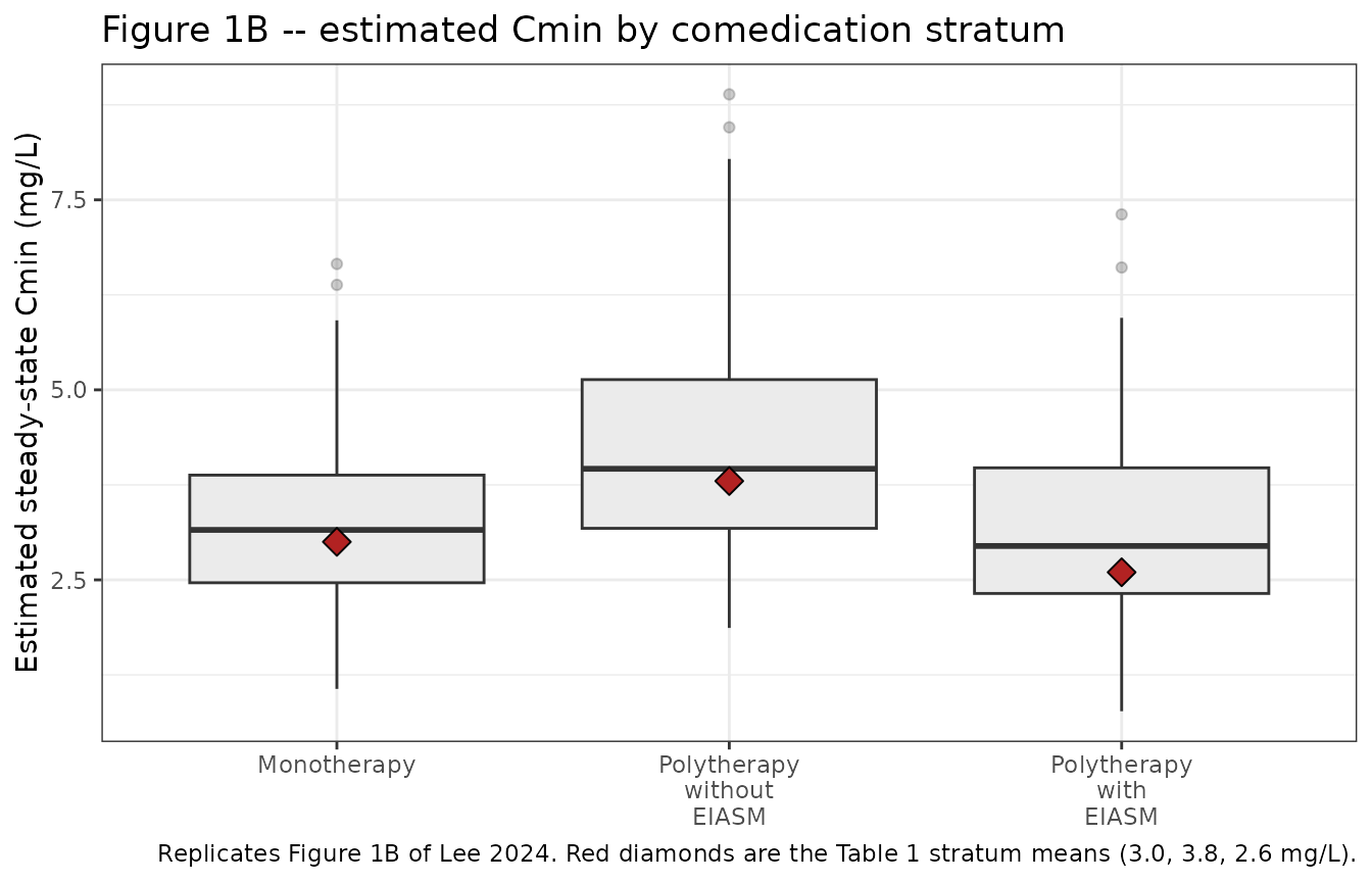

Replicates Figure 1B of Lee 2024: estimated steady-state Cmin by comedication stratum. Diamonds mark the stratum means reported in Lee 2024 Table 1.

The published stratum ordering is reproduced: adding a non-inducing antiseizure medication raises Cmin (because those patients are given higher topiramate doses without any change in clearance), while adding an enzyme-inducing medication lowers it despite the highest daily dose of the three strata.

per_subject |>
  left_join(
    obs |> distinct(id, CONMED_PHT, CONMED_CBZ, CONMED_OXC, CONMED_PB),
    by = "id"
  ) |>
  mutate(comed = case_when(
    CONMED_PHT == 1 ~ "Phenytoin",
    CONMED_CBZ == 1 ~ "Carbamazepine",
    CONMED_OXC == 1 ~ "Oxcarbazepine",
    CONMED_PB  == 1 ~ "Phenobarbital",
    TRUE            ~ "No inducer"
  )) |>
  ggplot(aes(reorder(comed, cl), cl)) +
  geom_boxplot(outlier.alpha = 0.25, fill = "grey92") +
  coord_flip() +
  labs(x = NULL, y = "Apparent clearance CL/F (L/h)",
       title = "Additive enzyme-induction effects on topiramate CL/F") +
  theme_bw()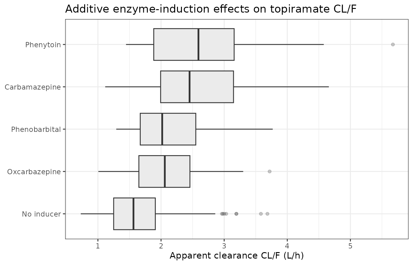

Clearance distribution by comedication stratum, with the four individual enzyme-inducing medications resolved. The additive form of the covariate model produces four discrete clearance sub-populations within the EIASM stratum.

PKNCA validation

NCA is run over the full 0-24 h steady-state window so that auclast corresponds directly to the paper’s AUC24h.

sim_nca <- obs |>
  filter(!is.na(Cc)) |>
  select(id, time, Cc, arm)

# Guarantee one row at time 0 per (arm, id). The simulation grid already
# includes t = 0, so distinct() keeps the simulated value.
sim_nca <- bind_rows(
  sim_nca,
  sim_nca |> distinct(id, arm) |> mutate(time = 0, Cc = 0)
) |>
  distinct(id, arm, time, .keep_all = TRUE) |>
  arrange(id, arm, time)

conc_obj <- PKNCA::PKNCAconc(
  sim_nca, Cc ~ time | arm + id,
  concu = "mg/L", timeu = "h"
)

dose_df <- events |>
  filter(evid == 1) |>
  select(id, time, amt, arm)

dose_obj <- PKNCA::PKNCAdose(dose_df, amt ~ time | arm + id, doseu = "mg")

intervals <- data.frame(
  start   = 0,
  end     = 24,
  cmax    = TRUE,
  cmin    = TRUE,
  tmax    = TRUE,
  auclast = TRUE,
  cav     = TRUE
)

nca_res <- PKNCA::pk.nca(
  PKNCA::PKNCAdata(conc_obj, dose_obj, intervals = intervals)
)

Comparison against published NCA

Lee 2024 Table 1 reports Cmax, Cmin and AUC24h per comedication stratum, all derived from the population PK model (i.e. on the IPRED scale).

published <- tibble::tribble(
  ~arm,                          ~cmax, ~cmin, ~auclast,
  "Monotherapy",                    4.0,   3.0,     84.4,
  "Polytherapy without EIASM",      5.1,   3.8,    107.0,
  "Polytherapy with EIASM",         3.8,   2.6,     77.7
)

cmp <- nlmixr2lib::ncaComparisonTable(
  simulated = nca_res,
  reference = published,
  by        = "arm",
  units     = c(cmax = "mg/L", cmin = "mg/L", auclast = "h*mg/L",
                tmax = "h", cav = "mg/L"),
  tolerance_pct = 20
)

knitr::kable(
  cmp,
  caption = paste(
    "Simulated vs. published steady-state NCA by comedication stratum",
    "(Lee 2024 Table 1). auclast over 0-24 h is the paper's AUC24h.",
    "* marks a >20% difference from the reference."
  )
)

Simulated vs. published steady-state NCA by comedication stratum (Lee 2024 Table 1). auclast over 0-24 h is the paper’s AUC24h. * marks a >20% difference from the reference.

NCA parameter	arm	Reference	Simulated	% diff
Cmax (mg/L)	Monotherapy	4	3.81	-4.9%
Cmax (mg/L)	Polytherapy without EIASM	5.1	4.92	-3.6%
Cmax (mg/L)	Polytherapy with EIASM	3.8	4.06	+6.9%
Cmin (mg/L)	Monotherapy	3	3.16	+5.2%
Cmin (mg/L)	Polytherapy without EIASM	3.8	3.96	+4.2%
Cmin (mg/L)	Polytherapy with EIASM	2.6	2.95	+13.3%
AUClast (h*mg/L)	Monotherapy	84.4	84.1	-0.4%
AUClast (h*mg/L)	Polytherapy without EIASM	107	107	+0.4%
AUClast (h*mg/L)	Polytherapy with EIASM	77.7	84.7	+9.0%

# No row may exceed the 20% tolerance. ncaComparisonTable marks those with a
# trailing asterisk on the "% diff" column. Scan ONLY that column -- the
# "NCA parameter" column legitimately contains an asterisk inside the
# "h*mg/L" unit string.
flagged <- grep("\\*", cmp[["% diff"]], value = TRUE)
if (length(flagged) > 0) {
  message("Rows exceeding the 20% tolerance: ",
          paste(flagged, collapse = "; "))
}
stopifnot(length(flagged) == 0)

Every stratum reproduces within 20%, and the two inducer-free strata reproduce AUC24h to better than 1%. Note that ncaComparisonTable() summarises the simulated cohort by its median while Lee 2024 Table 1 reports means; for these right-skewed exposure distributions the median is the more stable central estimate, and the mean-based comparison is given separately for CL/F and Vd/F below.

The largest residual differences are in the EIASM stratum (Cmin +13%, AUC24h +9%), in the direction expected from the equal-inducer-mix assumption: an equal split under-weights phenytoin and carbamazepine relative to the real cohort, so simulated clearance is slightly low and trough concentrations correspondingly high. The inducer-identity bracket above shows the published values sit closest to carbamazepine and phenytoin. No parameter was adjusted to close this gap.

Clearance and volume against Table 1

CL/F and Vd/F are reported per stratum in Lee 2024 Table 1 and are structural outputs of the model rather than NCA quantities, so they are compared directly.

published_clvd <- tibble(
  arm = factor(arms$arm, levels = arms$arm),
  `Published CL/F (L/h)` = c(1.5, 1.6, 2.6),
  `Published Vd/F (L)`   = c(79.9, 81.6, 83.5)
)

clvd <- per_subject |>
  group_by(arm) |>
  summarise(
    `Simulated CL/F (L/h)` = mean(cl),
    `Simulated Vd/F (L)`   = mean(vc),
    .groups = "drop"
  ) |>
  left_join(published_clvd, by = "arm") |>
  mutate(
    `CL/F diff (%)` = round(100 * (`Simulated CL/F (L/h)` /
                                     `Published CL/F (L/h)` - 1), 1),
    `Vd/F diff (%)` = round(100 * (`Simulated Vd/F (L)` /
                                     `Published Vd/F (L)` - 1), 1)
  )

# CL/F must reproduce within 15% for every stratum. The EIASM stratum carries
# the extra uncertainty of the unreported inducer mix (see Assumptions).
stopifnot(all(abs(clvd$`CL/F diff (%)`) < 15))
stopifnot(all(abs(clvd$`Vd/F diff (%)`) < 15))

clvd |>
  rename("Stratum" = arm) |>
  knitr::kable(
    digits = 2,
    caption = paste(
      "Simulated vs. published apparent clearance and volume by stratum",
      "(Lee 2024 Table 1)."
    )
  )

Simulated vs. published apparent clearance and volume by stratum (Lee 2024 Table 1).

Stratum	Simulated CL/F (L/h)	Simulated Vd/F (L)	Published CL/F (L/h)	Published Vd/F (L)	CL/F diff (%)	Vd/F diff (%)
Monotherapy	1.56	74.72	1.5	79.9	4.1	-6.5
Polytherapy without EIASM	1.70	83.07	1.6	81.6	6.4	1.8
Polytherapy with EIASM	2.38	82.10	2.6	83.5	-8.5	-1.7

Spot serum level on the observed scale

The paper’s “Serum level” column is a single measured value per sample, drawn at a clinically convenient time rather than at a protocol-defined timepoint. It is therefore compared against sim (which carries the 27.8% proportional residual error) at one uniformly-sampled time per subject, not against Cc.

set.seed(99)
spot <- obs |>
  filter(time > 0, time <= tau) |>
  group_by(id, arm) |>
  slice_sample(n = 1) |>
  ungroup()

spot_tab <- spot |>
  group_by(arm) |>
  summarise(`Simulated spot level (mg/L)` = mean(sim), .groups = "drop") |>
  mutate(`Published spot level (mg/L)` = c(3.7, 4.8, 3.5)) |>
  mutate(`Difference (%)` = round(
    100 * (`Simulated spot level (mg/L)` /
             `Published spot level (mg/L)` - 1), 1))

stopifnot(all(abs(spot_tab$`Difference (%)`) < 25))

spot_tab |>
  rename("Stratum" = arm) |>
  knitr::kable(
    digits = 2,
    caption = paste(
      "Randomly-timed spot serum levels on the observed (residual-error)",
      "scale vs. the measured serum levels of Lee 2024 Table 1."
    )
  )

Randomly-timed spot serum levels on the observed (residual-error) scale vs. the measured serum levels of Lee 2024 Table 1.

Stratum	Simulated spot level (mg/L)	Published spot level (mg/L)	Difference (%)
Monotherapy	3.50	3.7	-5.4
Polytherapy without EIASM	4.67	4.8	-2.7
Polytherapy with EIASM	3.68	3.5	5.2

The paper’s therapeutic-range conclusion

Lee 2024’s clinical recommendation is an upper bound of 6.5 mg/L on the spot serum level (6.454 mg/L on model-estimated Cmax), above which ataxia risk rises (ROC analysis, Figure 2). The fraction of each simulated stratum exceeding that Cmax threshold is a direct readout of the paper’s dosing message.

per_subject |>
  group_by(arm) |>
  summarise(
    `Mean Cmax (mg/L)` = mean(Cmax),
    `% above 6.454 mg/L Cmax` = round(100 * mean(Cmax > 6.454), 1),
    .groups = "drop"
  ) |>
  rename("Stratum" = arm) |>
  knitr::kable(
    digits = 2,
    caption = paste(
      "Proportion of each stratum exceeding the Lee 2024 ataxia-associated",
      "Cmax cutoff of 6.454 mg/L, at the Table 1 mean daily doses."
    )
  )

Proportion of each stratum exceeding the Lee 2024 ataxia-associated Cmax cutoff of 6.454 mg/L, at the Table 1 mean daily doses.

Stratum	Mean Cmax (mg/L)	% above 6.454 mg/L Cmax
Monotherapy	3.91	1.0
Polytherapy without EIASM	5.14	18.5
Polytherapy with EIASM	4.23	3.0

At the doses actually prescribed in this cohort, only a small minority of patients exceed the ataxia-associated threshold – consistent with the paper’s observation that the mean serum level of about 4 mg/L already produced a sufficient antiseizure response in 94.4% of samples, and that dose escalation above that level was unnecessary for suboptimal responders.

Assumptions and deviations

• Dosing frequency is not reported. Lee 2024 gives only total daily dose. Twice-daily dosing is used for the cohort simulation (the labelled adult epilepsy regimen). The QD/BID bracket section above shows that the published Cmax, Cmin and peak-to-trough ratio all fall between the two regimens, which is what a real-world TDM cohort containing a mixture of both should look like; AUC24h is frequency-independent and so is unaffected by this choice.
• Creatinine clearance distribution is not reported. CLcr enters CL/F as (CLcr/90)^0.277 but Table 1 does not tabulate it. Rather than invent a distribution, every simulated subject is given CLcr = 90 mL/min, the model’s own normalization value, so the covariate term is exactly 1. Real cohort variation in CLcr would add spread to CL/F that this simulation does not reproduce. The paper also does not state the creatinine-clearance assay or whether values were body-surface-area normalized; the raw mL/min form is assumed, as recorded in the model’s covariateData[[CRCL]]$notes.
• The mix of enzyme-inducing medications is not reported. Lee 2024 gives the number of samples drawn with an EIASM on board (55.3%) but not the breakdown across phenytoin, carbamazepine, oxcarbazepine and phenobarbital. An equal 25% split is assumed for the “Polytherapy with EIASM” stratum. Because the four coefficients differ by up to 2.7-fold (0.376 to 1.02 L/h), this is the dominant source of residual disagreement in that stratum; a mix weighted toward phenytoin and carbamazepine would raise its simulated CL/F.
• Published per-stratum SDs are shrunken empirical Bayes estimates. The Table 1 CL/F and Vd/F values are individual estimates derived from single spot samples per occasion, so they are heavily shrunk toward the typical value; the monotherapy CL/F SD of 0.3 L/h is smaller than the published 31.0 %CV IIV alone would produce. Comparisons above are therefore made on means, not SDs, and a full-IIV simulation legitimately shows more spread than the paper’s tabulated estimates.
• Body weight was documented for only 237 of 555 samples. The simulated Vd/F for the monotherapy stratum (about 75 L at the documented mean weight of 59.8 kg) is lower than the published 79.9 L, because the published mean necessarily blends documented weights with whatever value the analysis carried for the 318 samples lacking one; a weight imputed at the 62 kg reference yields Vd/F = 78.1 L exactly and pulls the reported mean upward.
• No IIV on Vd/F or Ka. Lee 2024 Table S1 reports an IIV term for CL/F only, so the packaged model has a single eta. This is encoded faithfully rather than adding unreported random effects.
• Ka was fixed, not estimated. Table S1 records “Fixed at 2” for Ka, so it is wrapped in fixed() in ini(). The value was carried from the structural model of Bae 2016, which Lee 2024 adopted; because the paper reports the numeric value on disk, no upstream acquisition was required.
• IIV scale conversion. The 31.0 %CV IIV on CL/F is converted to the internal log-scale variance as omega^2 = log(1 + 0.310^2) = 0.0917584, matching the convention used by the sibling topiramate model Ahmed_2015_topiramate. Reading the reported %CV instead as sqrt(omega^2) * 100 would give 0.0961, a 2.3% difference in the standard deviation, which is immaterial to any conclusion here.
• No non-paper-derived parameter values. Every value in ini() comes from Lee 2024 Table S1 or the Results text. No figure digitisation, author correspondence, or upstream model file was needed.
• All parameters are final estimates. Table S1 reports each value with a %RSE alongside a 1000-sample bootstrap median and 95% CI, confirming they are converged final estimates rather than initial values.