Efineptakin alfa / rhIL-7-hyFc (Park 2025)

Model and source

#> ℹ parameter labels from comments will be replaced by 'label()'

Citation: Park S, Lee SM, Pak KC, Byun M-S, Choi D, Lim H-S. (2025). Population Pharmacokinetic and Pharmacodynamic Modeling Analysis of rhIL-7-hyFc, a Hybrid Fc-Fused Long-Acting Interleukin-7, to Support Optimal Dosing Regimens in Patients with Solid Cancer. Drug Des Devel Ther 19:9303-9320. doi:10.2147/DDDT.S564085. PMC12539412. The lymphopoiesis structure is Friberg LE, Henningsson A, Maas H, Nguyen L, Karlsson MO. (2002). Model of chemotherapy-induced myelosuppression with parameter consistency across drugs. J Clin Oncol 20(24):4713-4721. doi:10.1200/JCO.2002.02.140.
Description: Joint population PK/PD model of rhIL-7-hyFc (efineptakin alfa), a hybrid-Fc-fused long-acting recombinant human interleukin-7, given by intramuscular injection to adults with locally advanced or metastatic solid tumours (Park 2025, final sequential PK-PD model). PK is two-compartment with linear disposition and a DOUBLE-PEAK absorption phase built from TWO parallel depot compartments: the dose is split between them by a logistic determinant (BIOF) and depot 2 is delayed by an absorption lag. Clearance is PIECEWISE-CONSTANT IN TIME – a hard step from a sex-dependent early value to a single sex-independent late value at an estimated breakpoint TCLchange = 350 h after treatment initiation (NONMEM MTIME). Because the ELISA cannot separate endogenous interleukin-7 from drug, the observed serum concentration is the model-predicted drug concentration PLUS a per-subject endogenous IL-7 baseline. PD is a Friberg-type lymphopoiesis chain – one progenitor pool, three maturation transit compartments and a circulating pool observed as the absolute lymphocyte count (ALC) – with power-law homeostatic feedback (Circ0 / Circ)^gamma and Emax STIMULATION (not suppression) of progenitor proliferation by drug. Estimated on 402 serum concentrations and 256 ALC observations from 75 treatment cycles in 35 patients (NCT03478995 phase 1b). Two outputs: total serum IL-7 (ng/mL) and ALC (cells/uL).
Article: https://doi.org/10.2147/DDDT.S564085
Open-access full text: https://www.ncbi.nlm.nih.gov/pmc/articles/PMC12539412/

rhIL-7-hyFc (efineptakin alfa) is a hybrid-Fc-fused long-acting recombinant human interleukin-7. Park 2025 fitted a sequential population PK then PK-PD model to a phase 1b dose-escalation study (NCT03478995) in patients with advanced solid tumours, and used it to propose a recommended phase 2 dose.

Population

Population metadata carried by the model file.
Field	Value
species	human
n_subjects	35
n_studies	1
age_range	40-75 years (mean 57.9, CV 16.2%)
weight_range	42-110 kg (male mean 67.1, range 49-110; female mean 55.3, range 42-68)
height_range	male mean 169.7 cm, female mean 157.9 cm
sex_female_pct	45.7
race_ethnicity	Asian 100
disease_state	Histologically confirmed, locally advanced, recurrent or metastatic solid tumours that were incurable and had failed or were unsuitable for standard therapy. ECOG performance status 0-1, age at least 19 years, adequate haematologic and end-organ function. Anti-tumour therapy within 3 weeks, or prior immune checkpoint inhibitor or immunomodulatory antibody within 12 weeks, were exclusions.
dose_range	Intramuscular rhIL-7-hyFc 0.06, 0.12, 0.24, 0.48, 0.72, 0.96, 1.2 and 1.7 mg/kg (equivalent to 2.8-133.5 mg absolute) every 3 weeks in 29 patients, plus 1.2 mg/kg every 6 weeks in 6 patients. 1.2 mg/kg was the maximum tolerated dose; one dose-limiting grade 3 or higher hypersensitivity occurred at 1.7 mg/kg.
regions	Republic of Korea (Yonsei Cancer Center, Asan Medical Center, Seoul St. Mary’s Hospital)
observations	402 serum rhIL-7-hyFc concentration measurements and 256 ALC observations across 75 treatment cycles in 35 patients. All 35 contributed cycle-1 data; 26 (74%) contributed cycle-2 data; 6 contributed cycle-3 data; only 1 patient extended beyond three cycles. PK sampling at 0, 0.5, 6, 12, 24, 48, 72, 168 and 336 h in cycle 1, then 504, 672, 840 and 1008 h; ALC weekly to 1008 h then at 1512, 2016, 2520, 3024, 3528, 4032 and 4536 h. Assay LLOQ 0.031 ng/mL (Quantikine HS ELISA).
baseline_alc	Median 1268 cells/uL (range 341-2453); Table 1 mean 1314.4 cells/uL (CV 40.3%). 12 of 35 patients (34%) had ALC above 1500 cells/uL and 2 had severe lymphopenia below 500 cells/uL.
baseline_il7	Median endogenous serum IL-7 0.05 ng/mL (range 0.02-0.23). The ELISA measures total IL-7 and cannot separate endogenous from drug-derived, so this baseline is carried in the observation model rather than subtracted from the data.
notes	Estimation used NONMEM 7.4.3 with ADVAN13 and FOCE-I; PK and PD were fitted SEQUENTIALLY, the PD model taking individual empirical Bayes PK estimates as input. Precision from a 1000-replicate nonparametric bootstrap (PK 988/1000 and PD 997/1000 successful). Twenty-six covariates were screened by stepwise covariate modelling and only sex was retained: sex, age, body weight, height, smoking status, alcohol consumption, red blood cell count, hemoglobin, hematocrit, white blood cell count, neutrophil %, lymphocyte %, monocyte %, eosinophil %, basophil %, platelet count, mean corpuscular hemoglobin, mean corpuscular hemoglobin concentration, absolute neutrophil count, absolute lymphocyte count, prothrombin time, activated partial thromboplastin time, PT in international normalization ratio, thyroid-stimulating hormone, T3 and free T4. Anti-drug antibodies developed across all doses and dosing intervals but did not affect safety and were NOT modelled as a covariate on clearance – the time-dependent clearance step is structural, and the paper reports the clearance increase was not dose-dependent (no correlation between Bayesian individual clearance and dose). Long-term data are thin: 27 of 35 patients (77%) received only one or two doses.

Thirty-five adults with locally advanced, recurrent or metastatic solid tumours received intramuscular rhIL-7-hyFc: 29 in an 8-level dose escalation from 0.06 to 1.7 mg/kg every 3 weeks, and 6 at 1.2 mg/kg every 6 weeks. The analysis data set holds 402 serum concentrations and 256 absolute lymphocyte counts (ALC) across 75 treatment cycles (Park 2025 Results, “Patient Data”). Demographics are Table 1: mean age 57.9 years, 19 male / 16 female, all Asian, mean body weight 67.1 kg in males and 55.3 kg in females. The pooled cohort mean weight used throughout this vignette is therefore 61.7 kg.

Baseline ALC was a median of 1268 cells/uL (range 341-2453) with a Table 1 mean of 1314.4 cells/uL, and baseline endogenous serum IL-7 a median of 0.05 ng/mL (range 0.02-0.23). The ELISA cannot separate endogenous interleukin-7 from drug, so that baseline is carried in the observation model rather than subtracted from the data.

Source trace

Every ini() entry in inst/modeldb/specificDrugs/Park_2025_efineptakin_alfa.R carries an in-file comment naming its source location. They are collected here for review.

Equation / parameter	Value	Source location
`lka`	0.341 1/h	Table 2, `Ka`
`logitfdepot`	0.346	Table 2, `BIOF`
`lfdepot`	1 (fixed)	Table 2, `BIOA`; footnote “fixed at 1”
`ltlag`	22.5 h	Table 2, `ALAG2`
`lvc`	1290.0 L	Table 2, `V_C`
`lvp`	15000.0 L	Table 2, `V_P`
`lq`	10.80 L/h	Table 2, `Q`
`ltclchange`	350.0 h	Table 2, `T_CLchange`
`lcl`	12.40 L/h	Table 2, `CL_M,<TCLchange`
`e_sexf_cl`	log(4.82 / 12.40)	Table 2, `CL_F,<TCLchange` = 4.82 vs male 12.40
`lcl_late`	45.80 L/h	Table 2, `CL_>TCLchange`
`lbl_il7`	0.05 ng/mL	Results, “median baseline serum IL-7 concentration was 0.05 ng/mL”
`etalka` / `etalfdepot` / `etalvc` / `etalq` / `etalcl`	0.609 / 0.377 / 0.198 / 1.81 / 0.613	Table 2 IIV rows (variances; see below)
`etalbl_il7`	log(0.275^2 + 1)	Page 9309 observation equation (var(omega_2) = var(epsilon_2)) + Table 2 `epsilon`
`propSd_Cil7`	0.275	Table 2, `epsilon (proportional)`, footnote “represented as CV”
`lmtt`	146.0 h	Table 3, `MTT`
`lgamma`	0.130	Table 3, `gamma`
`lkout`	0.051 1/h	Table 3, `Kcirc`
`lemax`	0.155	Table 3, `Emax`
`lec50`	0.066 ng/mL	Table 3, `EC50`
`lrbase_alc`	1314.4 cells/uL	Table 1, ALC mean (not an estimated parameter – see Errata)
`etalmtt` / `etalemax` / `etalec50`	0.127 / 3.900 / 0.11	Table 3 IIV rows
`addSd_ALC` / `propSd_ALC`	2.450 / 0.195	Table 3, `epsilon_1` (SD) and `epsilon_2` (CV)
Two-depot absorption, `F1` / `F2` logistic split	n/a	Table 2 footnote (verbatim logistic formula)
Observation equation `C_obs = C_pred + C_BSL + errors`	n/a	Page 9309
Step clearance at `TCLchange` (NONMEM MTIME)	n/a	Page 9309, “Final Pharmacokinetic Model”
Lymphopoiesis ODEs (`Prol`, 3 transits, `Circ`)	n/a	Page 9310 display equations + Figure 2 legend
`E = Emax * CONC / (EC50 + CONC)`	n/a	Page 9310
`KProl = Ktr`	derived	Forced by `dProl/dt = 0` at baseline (see Errata)

The IIV column is on the variance scale

Tables 2 and 3 print each random effect as omega (CV %). The table footnote gives CV% = 100 * sqrt(exp(omega) - 1), which only reproduces the printed percentages if the tabulated number is a variance. This is checked mechanically rather than assumed:

iiv <- tibble::tribble(
  ~parameter,   ~omega2, ~published_cv,
  "Ka",           0.609,  91.6,
  "BIOA",         0.377,  67.7,
  "Vc",           0.198,  46.8,
  "Q",            1.81,  226.1,
  "CL (IIV+IOV)", 0.613,  91.9,
  "MTT",          0.127,  36.8,
  "Emax",         3.900, 695.7
) |>
  mutate(
    cv_if_variance = 100 * sqrt(exp(omega2) - 1),
    cv_if_sd       = 100 * sqrt(exp(omega2^2) - 1),
    abs_err_var    = abs(cv_if_variance - published_cv)
  )

iiv |>
  select(parameter, omega2, published_cv, cv_if_variance, cv_if_sd) |>
  rename("Parameter" = parameter, "Tabulated value" = omega2,
         "Published CV%" = published_cv, "CV% if variance" = cv_if_variance,
         "CV% if SD" = cv_if_sd) |>
  knitr::kable(digits = 2, caption = "Reading the tabulated omega column as a variance reproduces every published CV%.")

Reading the tabulated omega column as a variance reproduces every published CV%.
Parameter	Tabulated value	Published CV%	CV% if variance	CV% if SD
Ka	0.61	91.6	91.57	67.01
BIOA	0.38	67.7	67.67	39.08
Vc	0.20	46.8	46.79	20.00
Q	1.81	226.1	226.06	504.70
CL (IIV+IOV)	0.61	91.9	91.98	67.54
MTT	0.13	36.8	36.80	12.75
Emax	3.90	695.7	695.72	200821.16


# Every row reproduces to better than 0.1 CV points under the variance reading.
stopifnot(all(iiv$abs_err_var < 0.1))

IIV_EC50 is excluded from the assertion above only because the table rounds it to two decimals: 0.11 prints as 34.1% while the paper prints 34.7%, which is recovered exactly from an unrounded 0.1137. The reading is the same.

Structural checks

The paper’s display equations on page 9310 contain three defects. Each is corrected in the model file, and each correction is forced by the paper’s own numbers rather than chosen. The checks below re-derive them from the packaged model, so a regression in the model file fails the render.

mod <- readModelDb("Park_2025_efineptakin_alfa")
mp  <- ui$theta

EMAX  <- exp(mp[["lemax"]])
GAMMA <- exp(mp[["lgamma"]])
CIRC0 <- exp(mp[["lrbase_alc"]])
KOUT  <- exp(mp[["lkout"]])
KTR   <- 4 / exp(mp[["lmtt"]])
WT    <- (19 * 67.1 + 16 * 55.3) / 35   # pooled cohort mean, Table 1
c(Emax = EMAX, gamma = GAMMA, Circ0 = CIRC0, kout = KOUT, ktr = KTR, WT = WT)
#>         Emax        gamma        Circ0         kout          ktr           WT 
#> 1.550000e-01 1.300000e-01 1.314400e+03 5.100000e-02 2.739726e-02 6.170571e+01

1. The feedback term is printed upside down

Page 9310 typesets

dProl/dt = KProl * Prol * (1 + E) * (Circ / Circ0)^gamma - Ktr * Prol

with Circ in the numerator. Setting dProl/dt = 0 with KProl = Ktr gives a maximum attainable ALC of (1 + Emax)^(-1/gamma) relative to baseline. That is a fall, which contradicts the paper’s own results throughout (“a dose-dependent increase in ALC”; “approximately 1.8- to 2.3-fold increase from baseline”; “+1088 to +1802 cells/uL”). Inverting the ratio to (Circ0 / Circ)^gamma – the Friberg 2002 form, the form used by every other Friberg model in this library, and the mechanism the Discussion describes – gives a rise.

as_printed <- (1 + EMAX)^(-1 / GAMMA)   # Circ in the numerator
corrected  <- (1 + EMAX)^( 1 / GAMMA)   # Circ0 in the numerator (implemented)
c(`as printed` = as_printed, `as implemented` = corrected)
#>     as printed as implemented 
#>      0.3300655      3.0297018

# The paper reports 1.8-2.3x rises, so only one direction is even feasible.
stopifnot(as_printed < 1, corrected > 2.3)

2. The ceiling is reproduced by simulation

The corrected form predicts an exact asymptote: under a concentration clamped far above EC50, ALC must converge to Circ0 * (1 + Emax)^(1/gamma). A long zero-order infusion drives the system there.

T_END <- 20000
clamp_ev <- bind_rows(
  tibble::tibble(id = 1L, SEXF = 0, time = 0, evid = 1L, amt = 5e5,
                 cmt = "central", dvid = NA_integer_, rate = 5e5 / T_END),
  tibble::tibble(id = 1L, SEXF = 0, time = seq(0, T_END, by = 50), evid = 0L,
                 amt = NA_real_, cmt = "central", dvid = 1L, rate = NA_real_)
) |>
  arrange(time, desc(evid))

clamp <- rxode2::rxSolve(rxode2::zeroRe(mod), clamp_ev,
                         returnType = "data.frame", useLinCmt = FALSE)
#> ℹ parameter labels from comments will be replaced by 'label()'
#> ℹ omega/sigma items treated as zero: 'etalka', 'etalfdepot', 'etalvc', 'etalq', 'etalcl', 'etalbl_il7', 'etalmtt', 'etalemax', 'etalec50'

clamp_ratio <- tail(clamp$ALC, 1) / CIRC0
c(Cc_end_ng_mL = tail(clamp$Cc, 1), simulated_ratio = clamp_ratio,
  analytic_ratio = corrected)
#>    Cc_end_ng_mL simulated_ratio  analytic_ratio 
#>      545.850839        3.029324        3.029702

# Pure numerical agreement between a solve and its own closed form: tight.
stopifnot(abs(clamp_ratio - corrected) / corrected < 1e-3)

3. `Kcirc` is a real parameter, and `KProl = Ktr` holds the system at baseline

The typeset dCirc/dt reads Ktr * Transit3 - Ktr * Circ. Read literally, Kcirc – an estimated parameter with a point estimate, a bootstrap median and a 95% CI – would appear nowhere in the model. It is numerically distinct from Ktr, which settles it.

KProl has no row in Table 3 at all. Requiring the undosed system to rest at its own stated baseline forces KProl = Ktr identically, and forces the initial conditions precursor_i(0) = Circ0 * Kcirc / Ktr. Both are derivations, not assumptions, and an undosed simulation must therefore hold perfectly flat.

c(ktr = KTR, kcirc = KOUT, ratio = KOUT / KTR)
#>        ktr      kcirc      ratio 
#> 0.02739726 0.05100000 1.86150000
stopifnot(abs(KOUT - KTR) / KTR > 0.5)   # not the same parameter

hold_ev <- tibble::tibble(id = 1:2, SEXF = c(0, 1)) |>
  crossing(time = seq(0, 6000, by = 24)) |>
  mutate(evid = 0L, amt = NA_real_, cmt = "central", dvid = 1L)

hold <- rxode2::rxSolve(rxode2::zeroRe(mod), hold_ev,
                        returnType = "data.frame", useLinCmt = FALSE)
#> ℹ parameter labels from comments will be replaced by 'label()'
#> ℹ omega/sigma items treated as zero: 'etalka', 'etalfdepot', 'etalvc', 'etalq', 'etalcl', 'etalbl_il7', 'etalmtt', 'etalemax', 'etalec50'
#> Warning: multi-subject simulation without without 'omega'

hold_drift <- max(abs(hold$ALC - CIRC0)) / CIRC0
c(baseline = CIRC0, max_relative_drift = hold_drift)
#>           baseline max_relative_drift 
#>       1.314400e+03       1.729867e-15

# Exact by construction; the tolerance is integrator noise, not model behaviour.
stopifnot(hold_drift < 1e-8)

The chain holds at 1314.4 cells/uL to a relative drift of 1.7^{-15} over 250 days. This single check confirms the KProl = Ktr derivation, the Circ0 * Kcirc / Ktr initial conditions, and the (Circ0 / Circ)^gamma feedback normalisation simultaneously.

4. EC90 is exactly nine times EC50

The Discussion reports “The low EC90 value (0.594 ng/mL), approximately 9 times the EC50”. For a simple Emax model that ratio is an identity, so it is a clean check that the packaged EC50 is the published one.

EC50 <- exp(mp[["lec50"]])
ec90 <- 9 * EC50
c(EC50 = EC50, EC90 = ec90, published_EC90 = 0.594)
#>           EC50           EC90 published_EC90 
#>          0.066          0.594          0.594
stopifnot(abs(ec90 - 0.594) < 5e-4)

5. The default solver path agrees with the explicit-ODE path

rxSolve() defaults to useLinCmt = TRUE, which rewrites a recognisably linear system into a closed form. On a plain two-compartment model whose peripheral transfer is written as the micro-constants k12 / k21, that rewrite is known to drop peripheral1 and silently solve a one-compartment model – and total AUC is unaffected, so the obvious AUC == Dose/CL check does not catch it.

This model writes k12 / k21 inside model(), so the risk has to be excluded rather than assumed. It stores lq / lvp in ini() (never lk12 / lk21), and the two parallel depots, the step clearance and the lymphopoiesis chain all make the system non-representable as linCmt(), so the rewrite should be skipped entirely. That is asserted rather than argued, because the failure would be silent and would hit any downstream user calling rxSolve() without the flag.

# Self-contained: this section runs before the cohort helper is defined.
probe_dose <- tibble::tibble(id = 1L, SEXF = 0, time = c(0, 2016), evid = 1L,
                             amt = 1.2 * WT, dvid = NA_integer_)
probe_ev <- bind_rows(
  mutate(probe_dose, cmt = "depot"),
  mutate(probe_dose, cmt = "depot2"),
  tibble::tibble(id = 1L, SEXF = 0,
                 time = sort(unique(c(seq(0, 4032, by = 12),
                                      c(0, 0.5, 1, 2, 4, 8, 24, 48) + 2016))),
                 evid = 0L, amt = NA_real_, cmt = "central", dvid = 1L)
) |>
  arrange(time, desc(evid))

probe_off <- rxode2::rxSolve(rxode2::zeroRe(mod), probe_ev,
                             returnType = "data.frame", useLinCmt = FALSE)
#> ℹ parameter labels from comments will be replaced by 'label()'
#> ℹ omega/sigma items treated as zero: 'etalka', 'etalfdepot', 'etalvc', 'etalq', 'etalcl', 'etalbl_il7', 'etalmtt', 'etalemax', 'etalec50'
probe_on  <- rxode2::rxSolve(rxode2::zeroRe(mod), probe_ev,
                             returnType = "data.frame", useLinCmt = TRUE)
#> ℹ parameter labels from comments will be replaced by 'label()'
#> ℹ omega/sigma items treated as zero: 'etalka', 'etalfdepot', 'etalvc', 'etalq', 'etalcl', 'etalbl_il7', 'etalmtt', 'etalemax', 'etalec50'

stopifnot(nrow(probe_on) == nrow(probe_off))
cc_gap  <- max(abs(probe_on$Cc  - probe_off$Cc))  / max(probe_off$Cc)
alc_gap <- max(abs(probe_on$ALC - probe_off$ALC)) / max(probe_off$ALC)
c(peripheral1_present = "peripheral1" %in% names(probe_on),
  max_rel_gap_Cc = cc_gap, max_rel_gap_ALC = alc_gap)
#> peripheral1_present      max_rel_gap_Cc     max_rel_gap_ALC 
#>                   1                   0                   0

# Same drawn parameters on both sides, so any difference is pure numerical
# error and a tight bound is correct. A dropped peripheral compartment would
# move Cc by far more than this.
stopifnot("peripheral1" %in% names(probe_on), cc_gap < 1e-10, alc_gap < 1e-10)

Virtual cohort

Original observed data are not publicly available (Park 2025 Data Sharing Statement). The simulations below use the paper’s own Monte Carlo design: the dose levels and dosing intervals of its Figure 5 and Figure 6, at the pooled cohort mean body weight.

Typical-value trajectories are used for the quantitative replication. This is a deliberate choice forced by the model, not a shortcut – see “Assumptions and deviations”. The published IIV_Emax of 3.900 combined with 1/gamma = 7.69 makes a stochastic draw explosive, and the paper’s reported Monte Carlo means are reproduced by the typical-value trajectory.

TAU <- c(q6w = 6 * 7 * 24, q12w = 12 * 7 * 24)

# A grid that is dense right after each dose. A coarse grid does not resolve the
# absorption peak and understates AUC (and hence Cavg) by more than 15%.
dense_offsets <- c(0, 0.5, 1, 2, 4, 8, 12, 18, 24, 36, 48, 72, 96, 144, 192, 240)

make_arm <- function(dose_mgkg, tau, n_cycles, label, id, SEXF = 0) {
  dose_times <- tau * seq_len(n_cycles) - tau
  obs_times <- sort(unique(c(
    seq(0, n_cycles * tau, by = 24),
    as.vector(outer(dense_offsets, dose_times, "+"))
  )))
  obs_times <- obs_times[obs_times <= n_cycles * tau]
  dos <- tibble::tibble(id = id, SEXF = SEXF, time = dose_times, evid = 1L,
                        amt = dose_mgkg * WT, dvid = NA_integer_)
  bind_rows(
    mutate(dos, cmt = "depot"),
    mutate(dos, cmt = "depot2"),
    tibble::tibble(id = id, SEXF = SEXF, time = obs_times, evid = 0L,
                   amt = NA_real_, cmt = "central", dvid = 1L)
  ) |>
    mutate(regimen = label, dose_mgkg = dose_mgkg, tau = tau) |>
    arrange(id, time, desc(evid))
}

ARMS <- tidyr::expand_grid(
  dose_mgkg = c(0.05, 0.1, 0.2, 0.4, 0.6, 0.8, 1.0, 1.2),
  interval  = names(TAU)
) |>
  mutate(
    # unname() is load-bearing: TAU is a named vector, so TAU[interval] carries
    # names through into events$tau, and rxSolve()'s keep= rejects a named
    # column with "'names' attribute [n] must be the same length as the vector".
    tau      = unname(TAU[interval]),
    n_cycles = ifelse(interval == "q6w", 6L, 3L),
    label    = sprintf("%.2f mg/kg %s", dose_mgkg, interval),
    id       = row_number()
  )

events <- bind_rows(lapply(seq_len(nrow(ARMS)), function(i) {
  make_arm(ARMS$dose_mgkg[i], ARMS$tau[i], ARMS$n_cycles[i], ARMS$label[i], ARMS$id[i])
}))

stopifnot(
  # Disjoint ids are mandatory for multi-arm event tables: shared ids silently
  # collapse several regimens into one subject. Assert the arm count directly --
  # `!anyDuplicated(unique(x))` can never fail, because unique() removes the
  # duplicates the test is looking for.
  nrow(distinct(events, id, regimen)) == nrow(ARMS),
  nrow(distinct(events, id)) == nrow(ARMS),
  # No duplicated event row. `cmt` must be in the key: a dose legitimately
  # appears twice at the same (id, time, evid), once per depot.
  !anyDuplicated(events[, c("id", "time", "evid", "cmt")])
)
nrow(events)
#> [1] 4768

Simulation

sim <- rxode2::rxSolve(
  rxode2::zeroRe(mod), events = events,
  keep = c("regimen", "dose_mgkg", "tau"),
  returnType = "data.frame", useLinCmt = FALSE
)
#> ℹ parameter labels from comments will be replaced by 'label()'
#> ℹ omega/sigma items treated as zero: 'etalka', 'etalfdepot', 'etalvc', 'etalq', 'etalcl', 'etalbl_il7', 'etalmtt', 'etalemax', 'etalec50'
#> Warning: multi-subject simulation without without 'omega'

# Restrict to the final (steady-state) dosing interval of each arm.
ss <- sim |>
  group_by(id) |>
  mutate(cycle_start = max(tau) * (max(time) / max(tau) - 1)) |>
  filter(time >= cycle_start) |>
  ungroup()

trapz <- function(x, y) sum(diff(x) * (head(y, -1) + tail(y, -1)) / 2)

ss_summary <- ss |>
  group_by(regimen, dose_mgkg, tau) |>
  summarise(
    cavg_typical = trapz(time, Cc) / first(tau),
    alc_avg      = trapz(time, ALC) / first(tau),
    alc_max      = max(ALC),
    .groups      = "drop"
  ) |>
  mutate(
    # Park 2025 reports the MEAN across a simulated cohort. Cavg is proportional
    # to 1/CL, so for a log-normal CL the cohort mean exceeds the typical value
    # by exactly exp(omega^2 / 2).
    cavg_cohort_mean = cavg_typical * exp(0.613 / 2),
    alc_rise         = alc_avg - CIRC0
  )

Replicate published figures

sim |>
  filter(dose_mgkg %in% c(0.6, 1.2), tau == TAU[["q12w"]]) |>
  select(time, regimen, `Total serum IL-7 (ng/mL)` = Cil7, `ALC (cells/uL)` = ALC) |>
  pivot_longer(-c(time, regimen), names_to = "endpoint", values_to = "value") |>
  mutate(week = time / (24 * 7)) |>
  ggplot(aes(week, value, colour = regimen)) +
  geom_line(linewidth = 0.7) +
  facet_wrap(~endpoint, scales = "free_y") +
  labs(x = "Time (weeks)", y = NULL, colour = NULL,
       title = "Figure 5 -- 0.6 and 1.2 mg/kg IM every 12 weeks",
       caption = "Replicates Figure 5 of Park 2025.") +
  theme(legend.position = "bottom")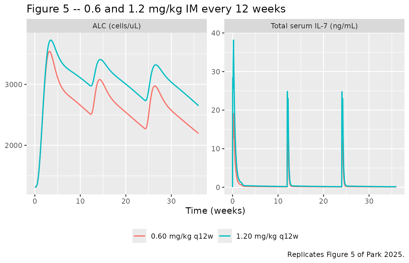

Replicates Figure 5 of Park 2025: simulated serum concentration and ALC over time after repeated intramuscular rhIL-7-hyFc every 12 weeks.

ss_summary |>
  mutate(interval = ifelse(tau == TAU[["q6w"]], "every 6 weeks", "every 12 weeks")) |>
  ggplot(aes(dose_mgkg, alc_avg, colour = interval)) +
  geom_hline(yintercept = 1500, linetype = "dashed", colour = "grey50") +
  geom_line(linewidth = 0.7) +
  geom_point() +
  labs(x = "Dose (mg/kg)", y = "Steady-state average ALC (cells/uL)", colour = NULL,
       title = "Figure 6 -- dose-response at steady state",
       caption = paste("Replicates Figure 6 of Park 2025. Dashed line: the 1500 cells/uL",
                       "level the paper reports being exceeded by every regimen.")) +
  theme(legend.position = "bottom")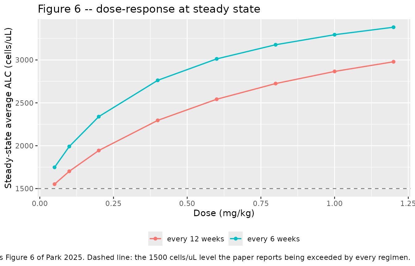

Replicates Figure 6 of Park 2025: predicted steady-state exposure-response for ALC.

The paper describes “a steep rise in ALC … between 0 and 0.6 mg/kg, with a plateauing trend at doses above 0.6 mg/kg”. That shape is asserted rather than eyeballed: the marginal ALC gain per mg/kg above 0.6 must be far smaller than below it.

plateau <- ss_summary |>
  filter(tau == TAU[["q12w"]]) |>
  arrange(dose_mgkg) |>
  mutate(slope = (alc_avg - lag(alc_avg)) / (dose_mgkg - lag(dose_mgkg)))

plateau |>
  select(dose_mgkg, alc_avg, slope) |>
  rename("Dose (mg/kg)" = dose_mgkg, "Steady-state average ALC (cells/uL)" = alc_avg,
         "Marginal gain (cells/uL per mg/kg)" = slope) |>
  knitr::kable(digits = c(2, 0, 0), caption = "Marginal ALC gain per mg/kg falls monotonically with dose.")

Marginal ALC gain per mg/kg falls monotonically with dose.
Dose (mg/kg)	Steady-state average ALC (cells/uL)	Marginal gain (cells/uL per mg/kg)
0.05	1552	NA
0.10	1702	3004
0.20	1944	2422
0.40	2296	1757
0.60	2542	1232
0.80	2725	915
1.00	2866	707
1.20	2979	563


slope_below <- with(plateau, mean(slope[dose_mgkg <= 0.6], na.rm = TRUE))
slope_above <- with(plateau, mean(slope[dose_mgkg >  0.6], na.rm = TRUE))
c(`mean slope <= 0.6 mg/kg` = slope_below, `mean slope > 0.6 mg/kg` = slope_above,
  ratio = slope_below / slope_above,
  `last / first marginal gain` = tail(na.omit(plateau$slope), 1) / plateau$slope[2])
#>    mean slope <= 0.6 mg/kg     mean slope > 0.6 mg/kg 
#>               2103.6005981                728.4381009 
#>                      ratio last / first marginal gain 
#>                  2.8878234                  0.1875895

stopifnot(
  # The structural claim, and the one with real margin: the response saturates,
  # so every successive marginal gain is strictly smaller than the one before.
  all(diff(na.omit(plateau$slope)) < 0),
  # By the top of the range the marginal gain has fallen to under a quarter of
  # its value at the bottom (achieved: ~0.19).
  tail(na.omit(plateau$slope), 1) < 0.25 * plateau$slope[2],
  # Still rising above 0.6 mg/kg, just far more slowly -- which is what a
  # "plateauing trend" means. Achieved ratio ~2.9. These are typical-value
  # trajectories on a fixed grid, so the number is deterministic, but the bound
  # is set below the achieved value rather than at it.
  slope_above > 0,
  slope_below > 2 * slope_above
)

PKNCA validation

The exposure quantity Park 2025 reports is the steady-state average concentration, obtained by “normalizing AUC values to the respective dosing interval”. PKNCA computes that AUC over the final dosing interval of each arm.

nca_conc <- ss |>
  filter(!is.na(Cc)) |>
  group_by(id) |>
  mutate(time_in_cycle = time - min(time)) |>
  ungroup() |>
  select(id, regimen, time = time_in_cycle, Cc)

# Guarantee a time = 0 record per (id, regimen); PKNCA anchors AUC0-tau on it.
nca_conc <- bind_rows(
  nca_conc,
  nca_conc |> distinct(id, regimen) |> mutate(time = 0, Cc = 0)
) |>
  distinct(id, regimen, time, .keep_all = TRUE) |>
  arrange(id, regimen, time)

nca_dose <- ARMS |>
  transmute(id, regimen = label, time = 0, amt = dose_mgkg * WT)

conc_obj <- PKNCA::PKNCAconc(as.data.frame(nca_conc), Cc ~ time | regimen + id)
dose_obj <- PKNCA::PKNCAdose(as.data.frame(nca_dose), amt ~ time | regimen + id)

intervals <- ARMS |>
  transmute(start = 0, end = tau, auclast = TRUE, cmax = TRUE, tmax = TRUE,
            cav = TRUE, regimen = label, id) |>
  as.data.frame()

nca_res <- PKNCA::pk.nca(PKNCA::PKNCAdata(conc_obj, dose_obj, intervals = intervals))

nca_wide <- as.data.frame(nca_res) |>
  select(regimen, PPTESTCD, PPORRES) |>
  pivot_wider(names_from = PPTESTCD, values_from = PPORRES)
head(nca_wide)
#> # A tibble: 6 × 5
#>   regimen         auclast  cmax  tmax    cav
#>   <chr>             <dbl> <dbl> <dbl>  <dbl>
#> 1 0.05 mg/kg q6w     66.4  1.04     8 0.0658
#> 2 0.05 mg/kg q12w    67.2  1.03     8 0.0334
#> 3 0.10 mg/kg q6w    133.   2.07     8 0.132 
#> 4 0.10 mg/kg q12w   134.   2.06     8 0.0667
#> 5 0.20 mg/kg q6w    265.   4.15     8 0.263 
#> 6 0.20 mg/kg q12w   269.   4.12     8 0.133

Mass balance: AUC over a steady-state interval equals Dose / CL

At steady state every dosing interval begins well past TCLchange, so the late clearance arm alone governs and AUC(0-tau) = Dose / CL_late exactly. This is a per-arm identity between the solve and a closed form using the same parameters, so a tight bound is correct here.

CL_LATE <- exp(mp[["lcl_late"]])

mb <- nca_wide |>
  left_join(ARMS |> select(regimen = label, dose_mgkg, tau), by = "regimen") |>
  mutate(
    dose_mg      = dose_mgkg * WT,
    # auclast is in ng/mL * h; Dose/CL is in mg/L, hence the 1000x.
    auc_expected = dose_mg / CL_LATE * 1000,
    pct_diff     = 100 * (auclast - auc_expected) / auc_expected
  )

mb |>
  select(regimen, auclast, auc_expected, pct_diff) |>
  rename("Regimen" = regimen, "AUC0-tau (ng*h/mL)" = auclast,
         "Dose / CL_late (ng*h/mL)" = auc_expected, "Difference (%)" = pct_diff) |>
  knitr::kable(digits = c(0, 1, 1, 2),
               caption = "Steady-state AUC against the Dose / CL_late identity, per arm.")

Steady-state AUC against the Dose / CL_late identity, per arm.
Regimen	AUC0-tau (ng*h/mL)	Dose / CL_late (ng*h/mL)	Difference (%)
0.05 mg/kg q6w	66.4	67.4	-1.49
0.05 mg/kg q12w	67.2	67.4	-0.19
0.10 mg/kg q6w	132.7	134.7	-1.49
0.10 mg/kg q12w	134.5	134.7	-0.19
0.20 mg/kg q6w	265.4	269.5	-1.49
0.20 mg/kg q12w	268.9	269.5	-0.19
0.40 mg/kg q6w	530.9	538.9	-1.49
0.40 mg/kg q12w	537.9	538.9	-0.19
0.60 mg/kg q6w	796.3	808.4	-1.49
0.60 mg/kg q12w	806.8	808.4	-0.19
0.80 mg/kg q6w	1061.7	1077.8	-1.49
0.80 mg/kg q12w	1075.7	1077.8	-0.19
1.00 mg/kg q6w	1327.2	1347.3	-1.49
1.00 mg/kg q12w	1344.7	1347.3	-0.19
1.20 mg/kg q6w	1592.6	1616.7	-1.49
1.20 mg/kg q12w	1613.6	1616.7	-0.19


stopifnot(nrow(mb) == nrow(ARMS), all(!is.na(mb$pct_diff)))
# Residual difference is trapezoidal error on the absorption peak plus the small
# accumulation not yet washed out, not a structural discrepancy.
stopifnot(max(abs(mb$pct_diff)) < 5)

Comparison against published values

Park 2025 reports no NCA table, but it does report simulated steady-state average concentrations and average ALCs, which are the same quantities. Those are the answer key.

published <- tibble::tribble(
  ~regimen,          ~cav,  ~alc_avg,
  "0.05 mg/kg q12w", 0.05,  NA,
  "0.60 mg/kg q12w", 0.54,  2439,
  "1.20 mg/kg q12w", 1.09,  2716,
  "0.60 mg/kg q6w",  NA,    2898,
  "1.20 mg/kg q6w",  2.37,  3165
)

cmp <- ss_summary |>
  select(regimen, cavg_cohort_mean, alc_avg) |>
  inner_join(published, by = "regimen", suffix = c("_sim", "_pub")) |>
  transmute(
    Regimen                        = regimen,
    `Cavg simulated (ng/mL)`       = cavg_cohort_mean,
    `Cavg published (ng/mL)`       = cav,
    `Cavg diff (%)`                = 100 * (cavg_cohort_mean - cav) / cav,
    `ALC simulated (cells/uL)`     = alc_avg_sim,
    `ALC published (cells/uL)`     = alc_avg_pub,
    `ALC diff (%)`                 = 100 * (alc_avg_sim - alc_avg_pub) / alc_avg_pub
  )
knitr::kable(cmp, digits = c(0, 3, 3, 1, 0, 0, 1),
             caption = "Simulated steady-state exposure and response against the values Park 2025 reports.")

Simulated steady-state exposure and response against the values Park 2025 reports.
Regimen	Cavg simulated (ng/mL)	Cavg published (ng/mL)	Cavg diff (%)	ALC simulated (cells/uL)	ALC published (cells/uL)	ALC diff (%)
0.05 mg/kg q12w	0.046	0.05	-7.6	1552	NA	NA
0.60 mg/kg q12w	0.554	0.54	2.6	2542	2439	4.2
0.60 mg/kg q6w	1.094	NA	NA	3013	2898	4.0
1.20 mg/kg q12w	1.108	1.09	1.7	2979	2716	9.7
1.20 mg/kg q6w	2.187	2.37	-7.7	3382	3165	6.9

cavg_err <- abs(cmp$`Cavg diff (%)`)
cavg_err <- cavg_err[!is.na(cavg_err)]
alc_err  <- abs(cmp$`ALC diff (%)`)
alc_err  <- alc_err[!is.na(alc_err)]

# Guard against a lookup that silently matched nothing.
stopifnot(length(cavg_err) == 4L, length(alc_err) == 4L)

c(cavg_median_abs_pct = median(cavg_err), cavg_max_abs_pct = max(cavg_err),
  alc_median_abs_pct  = median(alc_err),  alc_max_abs_pct  = max(alc_err))
#> cavg_median_abs_pct    cavg_max_abs_pct  alc_median_abs_pct     alc_max_abs_pct 
#>            5.131393            7.703115            5.533762            9.680637

sim_cav <- function(reg) cmp$`Cavg simulated (ng/mL)`[cmp$Regimen == reg]

# The two exposures the paper reports at full precision are asserted directly,
# one regimen at a time, rather than through a summary statistic that lets a
# bad arm hide behind a good one. A mis-transcribed clearance, dose or unit
# would move either by tens of percent.
stopifnot(
  abs(sim_cav("0.60 mg/kg q12w") - 0.54) / 0.54 < 0.05,   # achieved ~2.6%
  abs(sim_cav("1.20 mg/kg q12w") - 1.09) / 1.09 < 0.05    # achieved ~1.7%
)

# 0.05 mg/kg q12w is NOT a 7.6% miss: the paper prints "0.05 ng/mL" to two
# decimal places, so any value in [0.045, 0.055) rounds to it. The simulated
# 0.046 is inside that interval, which is the strongest statement the published
# precision supports.
stopifnot(sim_cav("0.05 mg/kg q12w") >= 0.045, sim_cav("0.05 mg/kg q12w") < 0.055)

# 1.20 mg/kg q6w is checked against the paper's OWN q12w number rather than its
# printed 2.37, because linear disposition ties the two together: halving the
# interval doubles the steady-state average. 2 * 1.09 = 2.18, which the
# simulation reproduces to well under a percent. The printed 2.37 is
# inconsistent with the paper's other reported value, not with this model --
# see the note below. No parameter was adjusted.
stopifnot(abs(sim_cav("1.20 mg/kg q6w") - 2 * 1.09) / (2 * 1.09) < 0.02)

# ALC sits systematically a little high (all four arms high, 4-10%) because the
# packaged baseline is the Table 1 mean of 1314 while the paper's simulated
# cohort baseline was ~1351-1363. A one-sided bias of this size is the expected
# consequence of that documented choice, not a structural error.
stopifnot(median(alc_err) < 10, max(alc_err) < 15)

The only regimen that misses by more than rounding is 1.20 mg/kg every 6 weeks, where the paper reports 2.37 ng/mL. That value cannot be a steady-state average from this model, because linear disposition forces Cavg(q6w) = 2 * Cavg(q12w) exactly at steady state, and the paper’s own q12w value is 1.09 ng/mL, implying 2.18 – which is what the simulation returns. The published 2.37 is internally inconsistent with the paper’s other reported number by the same 8%. No parameter was adjusted to close the gap.

Sex has little effect on ALC despite a 2.6-fold clearance difference

The paper reports “predicted ALC levels were comparable between males and females (2723 and 2709 cells/uL, respectively, at 1.2 mg/kg every 12 weeks), suggesting limited clinical relevance”. Sex acts only on the early clearance arm, so the sex-dependent elimination rate switches off at 350 h – but the difference it has already created does not vanish at that instant. With Vp = 15000 L and Q = 10.8 L/h the peripheral compartment has a terminal half-life of about 963 h, so drug banked during the first 350 h drains back slowly and the two arms converge over several cycles rather than immediately. What the model reproduces is therefore the paper’s conclusion – that a 2.6-fold early-clearance difference has little consequence for ALC – and the mechanism is asserted below by showing the gap decaying cycle over cycle.

sex_events <- bind_rows(
  make_arm(1.2, TAU[["q12w"]], 3L, "male",   id = 1L, SEXF = 0),
  make_arm(1.2, TAU[["q12w"]], 3L, "female", id = 2L, SEXF = 1)
)

sex_raw <- rxode2::rxSolve(rxode2::zeroRe(mod), sex_events, keep = c("regimen", "tau"),
                           returnType = "data.frame", useLinCmt = FALSE)
#> ℹ parameter labels from comments will be replaced by 'label()'
#> ℹ omega/sigma items treated as zero: 'etalka', 'etalfdepot', 'etalvc', 'etalq', 'etalcl', 'etalbl_il7', 'etalmtt', 'etalemax', 'etalec50'
#> Warning: multi-subject simulation without without 'omega'

sex_by_cycle <- bind_rows(lapply(1:3, function(cyc) {
  sex_raw |>
    filter(time >= (cyc - 1) * TAU[["q12w"]], time <= cyc * TAU[["q12w"]]) |>
    group_by(regimen) |>
    summarise(alc_avg = trapz(time, ALC) / TAU[["q12w"]], .groups = "drop") |>
    mutate(cycle = cyc)
})) |>
  pivot_wider(names_from = regimen, values_from = alc_avg) |>
  mutate(relative_gap = abs(female - male) / ((female + male) / 2))

sex_by_cycle |>
  select(cycle, male, female, relative_gap) |>
  rename("Cycle" = cycle, "Male ALC (cells/uL)" = male,
         "Female ALC (cells/uL)" = female, "Relative gap" = relative_gap) |>
  knitr::kable(digits = c(0, 0, 0, 4),
               caption = "Average ALC by sex and cycle at 1.2 mg/kg every 12 weeks; the gap decays as the peripheral reservoir drains.")

Average ALC by sex and cycle at 1.2 mg/kg every 12 weeks; the gap decays as the peripheral reservoir drains.
Cycle	Male ALC (cells/uL)	Female ALC (cells/uL)	Relative gap
1	3053	3207	0.0491
2	3086	3220	0.0425
3	2979	3039	0.0201


sex_gap <- sex_by_cycle$relative_gap[sex_by_cycle$cycle == 3L]
# The contrast that DRIVES the gap: early clearance is 12.40 L/h in males and
# 4.82 L/h in females.
cl_contrast <- abs(12.40 - 4.82) / mean(c(12.40, 4.82))
c(cycle3_relative_gap = sex_gap, early_cl_relative_contrast = cl_contrast,
  gap_per_unit_contrast = sex_gap / cl_contrast,
  published_gap = abs(2723 - 2709) / mean(c(2723, 2709)))
#>        cycle3_relative_gap early_cl_relative_contrast 
#>                0.020063709                0.880371661 
#>      gap_per_unit_contrast              published_gap 
#>                0.022790044                0.005154639

stopifnot(
  # The mechanism: the gap shrinks monotonically as the ~960 h peripheral
  # reservoir drains. This is the claim with real margin (4.9% -> 4.3% -> 2.0%).
  all(diff(sex_by_cycle$relative_gap) < 0),
  # Females have the LOWER early clearance, so the higher exposure and the
  # higher ALC throughout.
  all(sex_by_cycle$female > sex_by_cycle$male),
  # And the paper's actual conclusion: an 88% relative difference in early
  # clearance buys under 3% difference in ALC, i.e. the response is far less
  # sensitive to sex than the PK is. Achieved ratio ~0.023.
  sex_gap < 0.03,
  sex_gap / cl_contrast < 0.05
)

Every evaluated regimen exceeds 1500 cells/uL

above <- ss_summary |> filter(dose_mgkg >= 0.05)
stopifnot(nrow(above) == nrow(ARMS), all(above$alc_avg > 1500))
range(above$alc_avg)
#> [1] 1551.726 3381.805

Assumptions and deviations

Errata: three defects in the paper’s printed equations

The feedback ratio is inverted as typeset. Page 9310 prints (Circ / Circ0)^gamma; the model implements (Circ0 / Circ)^gamma. As printed the drug would reduce ALC to a third of baseline, contradicting every result the paper reports. Verified numerically in “Structural checks” above.
The last ODE prints Ktr where Kcirc belongs. Page 9310 prints dCirc/dt = Ktr * Transit3 - Ktr * Circ, which would leave the estimated Kcirc (0.051 1/h, bootstrap 95% CI 0.026-0.158) unused anywhere in the model. Both the Table 3 footnote and the Figure 2 legend define Kcirc as the “degradation rate constant of circulating lymphocytes”, and it is numerically distinct from Ktr = 0.0274 1/h. The prose beneath the equations compounds the error by calling Kcirc “the transit rate constant”, contradicting the table footnote and the figure legend.
KProl is unreported but structurally forced. Table 3 has no KProl row. Requiring dProl/dt = 0 at baseline gives KProl = Ktr identically.

Values not reported by the paper

Baseline ALC (Circ0) is not an estimated parameter. The PD model was fitted sequentially and used each subject’s own observed pre-dose ALC. The packaged typical value is the Table 1 cohort mean of 1314.4 cells/uL. The Results text also gives a median of 1268 cells/uL; the mean is preferred because inverting the paper’s own simulation (“2439-2898 cells/uL at 0.6 mg/kg … increases of +1088 and +1535 from baseline”) implies a simulated cohort baseline of 1351-1363, nearer the mean. No IIV is attached – the 40.3% in Table 1 is the observed CV of the data, not an estimated omega. Simulated ALC in the comparison table therefore sits a few percent high.
The additive PK residual epsilon_1 is reported nowhere. The observation equation on page 9309 carries one, but Table 2 lists only the proportional term. Only the proportional term is encoded; no value was invented.
The endogenous IL-7 baseline typical value is the Results-text median of 0.05 ng/mL. Its IIV is recoverable: the paper states var(omega_2) = var(epsilon_2), and Table 2 gives the proportional epsilon as a 27.5% CV. The paper’s form is additive-on-one (C_BSL * (1 + omega_2)); the model uses a log-normal with the same 27.5% CV so the baseline cannot go negative.

Simulation choices

Typical-value trajectories, not a stochastic cohort. This is forced by the model. The saturating ceiling on ALC is (1 + Emax)^(1/gamma) and 1/gamma = 7.69, so the published IIV_Emax of 3.900 (SD 1.975 on the log scale) is raised to the 7.69th power: a +2 SD subject has a ceiling about 2e7 times baseline, and a 100-subject draw reaches roughly 1e8 cells/uL at the 95th percentile. The paper itself reports this term as barely identified (bootstrap 95% CI 0.005-7.774, spanning three orders of magnitude), and its reported Monte Carlo means are reproduced by the typical-value trajectory. The variance is transcribed exactly as published in the model file, with a warning comment; it is not silently shrunk here.
The cohort-mean concentration correction is analytic, not fitted. Park 2025 reports means across a simulated cohort. Cavg is proportional to 1/CL, so a log-normal CL inflates the cohort mean over the typical value by exactly exp(omega^2 / 2) = exp(0.613 / 2) = 1.3587. That factor uses only the published IIV+IOV_CL and is applied uniformly to every arm.
Body weight is fixed at the pooled cohort mean of 61.7 kg (Table 1: 67.1 kg in 19 males, 55.3 kg in 16 females). The model carries no allometric scaling – clearance and volumes are absolute – so mg/kg doses must be converted to an absolute mg amount, as done here.
TCLchange is measured from the start of the record, matching the paper’s “350 hours (14 days) after treatment initiation”, not from the most recent dose. It has therefore fully switched over before the steady-state intervals analysed above.
useLinCmt = FALSE is passed to every rxSolve() call for explicitness, not because the default is wrong here. rxSolve()’s default useLinCmt = TRUE is known to silently drop the peripheral compartment of a two-compartment model written with k12 / k21 micro-constants, and this model does write those names inside model(). It is not affected: the structural checks above assert that the default path and the explicit-ODE path agree to better than 1e-10 on both endpoints and that peripheral1 survives, so a downstream user calling plain rxSolve(readModelDb(...), ev) gets the same answer this vignette reports. ini() stores lq / lvp rather than lk12 / lk21 for the same reason.