Posaconazole (Sime 2019)

Model and source

• Citation: Sime FB, Byrne CJ, Parker S, Stuart J, Butler J, Starr T, Pandey S, Wallis SC, Lipman J, Roberts JA. Population pharmacokinetics of total and unbound concentrations of intravenous posaconazole in adult critically ill patients. Crit Care. 2019;23(1):205. doi:10.1186/s13054-019-2483-9. PMCID PMC6554926. Structural model from Fig. 1 and Methods Eqs. 2-5; parameter estimates from Table 2; covariate model from Results ‘Pharmacokinetic model building’.
• Description: Two-compartment intravenous population PK model for posaconazole in critically ill adults, fitted SIMULTANEOUSLY to total and unbound plasma concentrations with explicit capacity-limited (Michaelis-Menten) albumin binding. The central compartment carries two states: a free posaconazole pool and an albumin-bound pool exchanging by second-order association (kon) and first-order dissociation (koff), giving the equilibrium isotherm Cbound = Bmax * Cfree / (KD + Cfree) with KD = koff / kon. Elimination and intercompartmental distribution both act on the UNBOUND concentration. Serum albumin sets the binding capacity Bmax = ALB * N * (MW_posaconazole / MW_albumin) * 1000 with N fixed to 1 binding site per albumin molecule, and body mass index scales the central volume linearly (V = Vtheta * BMI/24). Fitted NON-PARAMETRICALLY with the NPAG algorithm in Pmetrics; the Table 2 means are encoded as lognormal medians and the tabulated CV percentages as independent lognormal marginal variances. Residual unexplained variability is carried as fixed(0) because the selected Pmetrics error model was never published.
• Article: https://doi.org/10.1186/s13054-019-2483-9 (open access; PMCID PMC6554926)

No supplementary material accompanies this article; the model is fully specified by Fig. 1, Methods Eqs. 1-5 and Table 2 of the main text.

mod <- readModelDb("Sime_2019_posaconazole")
ui <- rxode2::rxode(mod)

# The model has THREE ODE states and TWO declared endpoints. Both facts are
# load-bearing for every simulation below, so assert them once here: a silent
# compartment renumbering would otherwise change every number in this vignette.
stopifnot(
  identical(ui$state, c("central", "complex", "peripheral1")),
  identical(ui$predDf$cond, c("Cc", "Cunbound"))
)

Population

Sime 2019 enrolled eight critically ill adults in the intensive care unit of the Royal Brisbane and Women’s Hospital (Australia) with presumed or confirmed invasive fungal infection. Each received a single 300 mg intravenous dose of posaconazole as a 90-minute infusion through a central venous catheter, on top of the antifungal therapy prescribed as usual care, and was sampled 14 times over 48 h. Ninety-three paired total and unbound plasma concentrations were measured by UHPLC-MS/MS.

The cohort was middle-aged (median 46 years, IQR 40-51), predominantly male (7 of 8), of median weight 68 kg (IQR 65-82) and median body mass index 22.6 kg/m^2 (IQR 20.2-29.7). It was markedly hypoalbuminaemic: median serum albumin 20 g/L (IQR 18-24), against a normal adult range of roughly 35-50 g/L. Renal function was broadly preserved (measured urinary creatinine clearance median 74 mL/min, IQR 53-109) and illness severity was substantial (median APACHE II 17 at ICU admission; median SOFA 5 on day 1). Baseline demographics are Sime 2019 Table 1.

The observed unbound fraction was median 0.55 percent (IQR 0.36-1.9), mean 0.65 percent (SD 0.39), coefficient of variation 58.5 percent: posaconazole is one of the most extensively protein-bound antifungals in clinical use, and that is what makes the total-versus-unbound distinction the subject of this paper.

The same information is available programmatically via rxode2::rxode(readModelDb("Sime_2019_posaconazole"))$population.

Model structure

Sime 2019 Fig. 1 shows a two-compartment disposition model in which the central compartment (volume V) carries two species: free posaconazole Cf(t) and albumin-bound posaconazole Cb(t), exchanging by a second-order association rate constant kon and a first-order dissociation rate constant koff. Both elimination (ke) and distribution to the peripheral compartment (kcp, kpc) act on the unbound species, which is why the tabulated ke and kcp are so large: scaled by the roughly 0.65 percent unbound fraction they give ordinary posaconazole disposition (checked numerically below).

The packaged model encodes exactly that figure:

d/dt(central)     = -kel*central - k12*central + k21*peripheral1 - bindflux
d/dt(complex)     =  bindflux
d/dt(peripheral1) =  k12*central - k21*peripheral1

bindflux          = kon*Cunbound*(bmax - Cbound)*vc - koff*complex
bmax              = ALB * N * (MW_posaconazole / MW_albumin) * 1000      (Eq. 3)

The stationary point of bindflux is the paper’s Eq. 2 isotherm Cbound = bmax * Cunbound / (KD + Cunbound) with KD = koff / kon (Eq. 4), and Cc = Cunbound + Cbound is Eq. 5 rearranged. The complex state is the registered TMDD drug-target complex compartment reused for a drug-protein complex; free albumin is not carried as a target state because only the aggregate capacity bmax is identified.

Source trace

Per-parameter provenance is recorded as an in-file comment beside each ini() entry in inst/modeldb/specificDrugs/Sime_2019_posaconazole.R. Collected here:

Equation / parameter	Value	Source location
lkel (Ke)	42.07 1/h	Table 2, row Ke (h-1), Mean column
lvc (V theta)	72.19 L	Table 2, row V theta (l), Mean column; Abstract rounds to 72 (43) L
lk12 (Kcp)	334.27 1/h	Table 2, row Kcp (h-1), Mean column
lk21 (Kpc)	0.37 1/h	Table 2, row Kpc (h-1), Mean column
lkon (Kon)	2820.35 L/mg/h	Table 2, row Kon (L/mg/h), Mean column
lkoff (Koff)	3897.40 1/h	Table 2, row Koff (h-1), Mean column
nalb (N)	1 (held fixed)	Methods, Eq. 3 definition list: “N was assumed to be 1.”
etalkel	0.27277	Table 2 Ke CV 56; omega^2 = log(0.56^2 + 1)
etalvc	0.30748	Table 2 V theta CV 60; omega^2 = log(0.60^2 + 1)
etalk12	0.40819	Table 2 Kcp CV 71; omega^2 = log(0.71^2 + 1)
etalk21	0.09176	Table 2 Kpc CV 31; omega^2 = log(0.31^2 + 1)
etalkon	0.05600	Table 2 Kon CV 24; omega^2 = log(0.24^2 + 1)
etalkoff	0.02225	Table 2 Koff CV 15; omega^2 = log(0.15^2 + 1)
propSd, propSd_Cunbound	0 (held fixed)	Not reported anywhere in the source; see Errata
Two-compartment structure with a bound central sub-pool	n/a	Fig. 1 and its legend
Cbound = bmax*Cunbound/(KD + Cunbound)	n/a	Eq. 2
bmax = ALB*N*(Mposa/MAlb)*1000	n/a	Eq. 3
KD = 1/KA = koff/kon	n/a	Eq. 4
Cc = Cunbound + Cbound	n/a	Eq. 5 (Cfree = Ctotal - Cbound)
vc = V theta * BMI / 24	n/a	Results, “Pharmacokinetic model building”
MW_posaconazole = 700.8 g/mol, MW_albumin = 66500 g/mol	n/a	Not printed in the source; standard physical constants, confirmed below against the paper’s own reported mean unbound fraction

Structural checks (typical individual)

These are deterministic: they use the typical individual (omega = NA) and compare the simulated model against closed-form quantities that follow from the published parameters. They are the tightest gates in this vignette.

# Published Table 2 values, restated here so the checks below are independent of
# the model file rather than reading their inputs out of it.
Ke <- 42.07
Vth <- 72.19
Kcp <- 334.27
Kpc <- 0.37
Kon <- 2820.35
Koff <- 3897.40
MW_POSA <- 700.8
MW_ALB <- 66500

KD <- Koff / Kon # Eq. 4
bmax_at <- function(alb) alb * 1 * (MW_POSA / MW_ALB) * 1000 # Eq. 3
fu_at <- function(alb) KD / (bmax_at(alb) + KD) # Discussion, "fu = KD/(Bmax + KD)"

c(KD_mg_per_L = KD, Bmax_at_ALB20 = bmax_at(20), fu_at_ALB20_pct = 100 * fu_at(20))
#>     KD_mg_per_L   Bmax_at_ALB20 fu_at_ALB20_pct 
#>       1.3818852     210.7669173       0.6513755

Check 1 – the reported mean unbound fraction falls out of Table 2

Sime 2019 reports a mean unbound fraction of 0.65 percent (Results, “Plasma protein binding”) and a median cohort albumin of 20 g/L (Table 1). Those two numbers were measured, not fitted, so reproducing the first from the second plus Table 2 is an independent consistency check on the whole binding block – and it is what pins the two molecular weights the paper defines symbolically but never prints.

fu_pred_pct <- 100 * fu_at(20)
# Paper: mean (SD) unbound fraction 0.65 (0.39) percent, from 93 measured pairs.
stopifnot(abs(fu_pred_pct - 0.65) < 0.02)
sprintf("predicted fu at ALB = 20 g/L: %.4f percent (paper reports 0.65 percent)", fu_pred_pct)
#> [1] "predicted fu at ALB = 20 g/L: 0.6514 percent (paper reports 0.65 percent)"

Check 2 – the kon/koff ODE reproduces the Eq. 2 isotherm

The packaged model integrates association and dissociation explicitly rather than imposing Eq. 2 algebraically. Because koff and kon*bmax are four to five orders of magnitude faster than every PK rate constant, the two species sit at quasi-equilibrium at all times, so the simulated Cbound must satisfy Eq. 2 to high precision. If it did not, the binding block would be misencoded.

one_subject <- function(dose = 300, ii = 24, ndose = 1, alb = 20, bmi = 24,
                        times = seq(0, 48, by = 0.25)) {
  dosing <- data.frame(
    id = 1L, time = seq(0, by = ii, length.out = ndose),
    amt = dose, rate = dose / 1.5, evid = 1L,
    cmt = "central", dvid = NA_integer_
  )
  obs <- data.frame(
    id = 1L, time = times, amt = NA_real_, rate = NA_real_, evid = 0L,
    cmt = "central", dvid = 1L
  )
  ev <- rbind(dosing, obs)
  ev$ALB <- alb
  ev$BMI <- bmi
  ev[order(ev$time, -ev$evid), ]
}

solve_typical <- function(ev) {
  # zeroRe() segfaults on models with two or more declared endpoints; omega = NA
  # and sigma = NA are the equivalent typical-value route. useLinCmt = FALSE is
  # required because rxode2's automatic linCmt rewrite corrupts the dvid map on
  # multi-endpoint models.
  rxode2::rxSolve(
    mod, ev,
    returnType = "data.frame", useLinCmt = FALSE,
    omega = NA, sigma = NA
  )
}

typ <- solve_typical(one_subject())
iso <- bmax_at(20) * typ$Cunbound / (KD + typ$Cunbound)
rel_err <- abs(typ$Cbound - iso) / pmax(typ$Cbound, 1e-12)

# Deterministic, not cohort-derived, so a tight bound is the right bound. The
# residual deviation is PHYSICAL rather than numerical: it is unchanged when the
# solver tolerances are tightened from (atol 1e-8, rtol 1e-6) to (1e-12, 1e-10),
# it peaks at 7.6e-4 at t = 0.25 h -- early in the 90-minute infusion, when the
# free pool is changing fastest and the finite-rate binding lags furthest behind
# its equilibrium -- and falls below 2.3e-4 once the infusion is over. A
# misencoded isotherm would be wrong by orders of magnitude, not parts per
# thousand.
worst_all <- max(rel_err[typ$time > 0])
worst_post <- max(rel_err[typ$time >= 2])
stopifnot(worst_all < 2e-3, worst_post < 1e-3)
sprintf(
  "max relative deviation of simulated Cbound from Eq. 2: %.3g overall, %.3g after the infusion",
  worst_all, worst_post
)
#> [1] "max relative deviation of simulated Cbound from Eq. 2: 0.000758 overall, 0.000225 after the infusion"

Check 3 – derived clearance, steady-state volume and terminal half-life

In the linear-binding regime the model occupies (Cunbound stays far below KD), the three micro-constants reduce to an ordinary two-compartment system with k10 = Ke * fu, k12 = Kcp * fu and k21 = Kpc. That gives closed forms for clearance, steady-state volume and the terminal disposition rate constant, none of which Sime 2019 prints – so this check both validates the encoding and shows that the very large tabulated rate constants are physiologically reasonable once the unbound fraction is applied.

fu20 <- fu_at(20)
k10 <- Ke * fu20
k12e <- Kcp * fu20
k21 <- Kpc
CL_closed <- k10 * Vth
Vss_closed <- Vth * (1 + k12e / k21)
lambda2 <- (k10 + k12e + k21 - sqrt((k10 + k12e + k21)^2 - 4 * k10 * k21)) / 2
thalf_closed <- log(2) / lambda2

# Same quantities recovered from the simulated typical profile.
trap <- function(t, v) sum(diff(t) * (head(v, -1) + tail(v, -1)) / 2)
tail_fit <- stats::lm(log(Cc) ~ time, data = subset(typ, time >= 30))
lambda2_sim <- -stats::coef(tail_fit)[["time"]]
auc_inf_sim <- trap(typ$time, typ$Cc) + utils::tail(typ$Cc, 1) / lambda2_sim
CL_sim <- 300 / auc_inf_sim

derived <- tibble::tibble(
  Quantity = c(
    "Clearance (L/h)", "Steady-state volume (L)", "Terminal half-life (h)"
  ),
  `Closed form` = c(CL_closed, Vss_closed, thalf_closed),
  Simulated = c(CL_sim, NA_real_, log(2) / lambda2_sim)
)
knitr::kable(derived, digits = 2, caption = "Derived disposition of the typical individual at ALB = 20 g/L, BMI = 24 kg/m2.")

Derived disposition of the typical individual at ALB = 20 g/L, BMI = 24 kg/m2.

Quantity	Closed form	Simulated
Clearance (L/h)	19.78	19.81
Steady-state volume (L)	497.01	NA
Terminal half-life (h)	19.04	19.05

# Deterministic identities: the simulated values differ from the closed forms
# only by trapezoidal error and the slight (< 1 percent) binding saturation.
stopifnot(
  abs(CL_sim / CL_closed - 1) < 0.02,
  abs((log(2) / lambda2_sim) / thalf_closed - 1) < 0.02
)

A clearance near 20 L/h, a steady-state volume near 500 L and a terminal half-life near 19 h sit squarely inside the published posaconazole range, which is the point: the Table 2 rate constants are not implausible, they simply multiply an unbound concentration.

Check 4 – mass balance

# Total drug in the body plus everything eliminated must equal the dose. The
# elimination flux is kel * central (kel acts on the free amount).
fine <- solve_typical(one_subject(times = seq(0, 48, by = 0.02)))
in_body <- utils::tail(fine$central + fine$complex + fine$peripheral1, 1)
eliminated <- trap(fine$time, Ke * fine$central)
stopifnot(abs((in_body + eliminated) / 300 - 1) < 0.005)
sprintf(
  "dose 300 mg; in body at 48 h %.1f mg + eliminated %.1f mg = %.1f mg",
  in_body, eliminated, in_body + eliminated
)
#> [1] "dose 300 mg; in body at 48 h 49.1 mg + eliminated 250.9 mg = 300.0 mg"

Virtual cohorts

Original observed data are not publicly available (the paper states the dataset is restricted by its ethics approval). The simulations below reproduce the paper’s own Monte Carlo dosing scenarios, which fix albumin and BMI at stated values rather than sampling a demographic distribution, so each “arm” is a covariate-homogeneous cohort of 200 subjects differing only in their random effects. Sime 2019 used 1000 subjects per scenario; 200 is the cap for this package’s vignettes, so probabilities carry a binomial standard error of about 3 percentage points near 80 percent – allowed for in every gate below.

# set.seed() seeds R's RNG, NOT rxode2's; and rxode2 partitions its streams per
# solver thread, so a CI runner with a different thread count draws a different
# cohort from the same source. Every assertion downstream is written to hold for
# any cohort this model can produce.
set.seed(20190606)
rxode2::rxSetSeed(20190606)

N_PER_ARM <- 200L

make_arm <- function(dose, ii, ndose, alb, bmi, label,
                     obs_times = c(0, 48), id_offset = 0L) {
  ids <- id_offset + seq_len(N_PER_ARM)
  dosing <- tidyr::expand_grid(
    id = ids,
    time = seq(0, by = ii, length.out = ndose)
  ) |>
    dplyr::mutate(
      amt = dose, rate = dose / 1.5, evid = 1L,
      cmt = "central", dvid = NA_integer_
    )
  obs <- tidyr::expand_grid(id = ids, time = obs_times) |>
    dplyr::mutate(
      amt = NA_real_, rate = NA_real_, evid = 0L,
      cmt = "central", dvid = 1L
    )
  dplyr::bind_rows(dosing, obs) |>
    dplyr::mutate(ALB = alb, BMI = bmi, arm = label) |>
    dplyr::arrange(id, time, dplyr::desc(evid))
}

solve_arm <- function(ev) {
  rxode2::rxSolve(
    mod, ev,
    keep = c("arm", "ALB", "BMI"),
    returnType = "data.frame", useLinCmt = FALSE, sigma = NA
  )
}

Replicate Figure 3 – albumin changes the total-trough PTA but not the unbound-trough PTA

Sime 2019 Fig. 3 simulates 300 mg given every 8 h (90-minute infusions) at a fixed BMI of 24 kg/m^2 and plots the probability of attaining a range of 48-hour trough targets, one curve per albumin level. Panel (a) uses total-concentration targets, panel (b) unbound-concentration targets. The paper’s claim is that the four albumin curves separate widely in panel (a) and collapse onto one another in panel (b) – the mechanistic statement that hypoalbuminaemia lowers the total trough while leaving the unbound trough essentially untouched.

alb_levels <- c(15, 25, 35, 45)
fig3_events <- dplyr::bind_rows(lapply(seq_along(alb_levels), function(i) {
  make_arm(
    dose = 300, ii = 8, ndose = 4, alb = alb_levels[i], bmi = 24,
    label = paste0("alb=", alb_levels[i], " g/L"),
    id_offset = (i - 1L) * N_PER_ARM
  )
}))
stopifnot(!anyDuplicated(unique(fig3_events[, c("id", "time", "evid")])))

fig3_sim <- solve_arm(fig3_events)
fig3_trough <- fig3_sim |>
  dplyr::filter(abs(time - 48) < 1e-9) |>
  dplyr::select(id, arm, ALB, Cc, Cunbound)
stopifnot(nrow(fig3_trough) == length(alb_levels) * N_PER_ARM)

total_targets <- c(0.175, 0.350, 0.500, 0.700, 1.000)
free_targets <- c(0.0011, 0.0023, 0.0033, 0.0045, 0.0065)

pta_curve <- function(df, column, targets, panel) {
  grid <- tidyr::expand_grid(this_arm = unique(df$arm), target = targets)
  grid$PTA <- vapply(seq_len(nrow(grid)), function(i) {
    mean(df[[column]][df$arm == grid$this_arm[i]] >= grid$target[i])
  }, numeric(1))
  grid$panel <- panel
  dplyr::rename(grid, arm = this_arm)
}

fig3 <- dplyr::bind_rows(
  pta_curve(fig3_trough, "Cc", total_targets, "a. Total trough target (mg/L)"),
  pta_curve(fig3_trough, "Cunbound", free_targets, "b. Unbound trough target (mg/L)")
)

ggplot(fig3, aes(target, PTA, colour = arm, shape = arm)) +
  geom_line() +
  geom_point() +
  geom_hline(yintercept = 0.8, linetype = "dashed") +
  facet_wrap(~panel, scales = "free_x") +
  scale_x_log10() +
  coord_cartesian(ylim = c(0, 1)) +
  labs(
    x = "Trough concentration target at 48 h (mg/L)", y = "PTA",
    colour = NULL, shape = NULL,
    title = "Figure 3 - PTA for 300 mg q8h x 4 at BMI 24, by serum albumin",
    caption = "Replicates Figure 3 of Sime 2019. Dashed line is the 80 percent PTA criterion."
  ) +
  theme(legend.position = "bottom")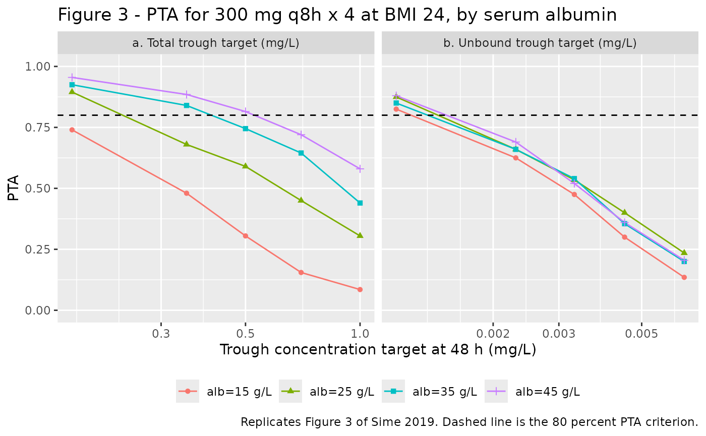

# Values read off the Fig. 3 panels of the published PDF by eye. They are
# approximate (roughly +/- 0.03 on the PTA axis) and are shown for visual
# comparison only -- the GATES below are on the paper's structural claims, not
# on these digitised numbers.
fig3_published <- tibble::tribble(
  ~panel_short, ~arm, ~target, ~PTA_paper,
  "total", "alb=15 g/L", 0.350, 0.40,
  "total", "alb=25 g/L", 0.350, 0.74,
  "total", "alb=35 g/L", 0.350, 0.89,
  "total", "alb=45 g/L", 0.350, 0.98,
  "total", "alb=15 g/L", 0.500, 0.22,
  "total", "alb=25 g/L", 0.500, 0.50,
  "total", "alb=35 g/L", 0.500, 0.74,
  "total", "alb=45 g/L", 0.500, 0.86,
  "free", "alb=15 g/L", 0.0023, 0.60,
  "free", "alb=25 g/L", 0.0023, 0.60,
  "free", "alb=35 g/L", 0.0023, 0.61,
  "free", "alb=45 g/L", 0.0023, 0.60,
  "free", "alb=15 g/L", 0.0033, 0.38,
  "free", "alb=25 g/L", 0.0033, 0.39,
  "free", "alb=35 g/L", 0.0033, 0.38,
  "free", "alb=45 g/L", 0.0033, 0.38
)

fig3_cmp <- fig3 |>
  dplyr::mutate(panel_short = ifelse(grepl("^a\\.", panel), "total", "free")) |>
  dplyr::inner_join(fig3_published, by = c("panel_short", "arm", "target")) |>
  dplyr::transmute(
    Panel = panel_short, Albumin = arm, Target = target,
    `PTA simulated` = PTA, `PTA read from Fig. 3` = PTA_paper,
    `Difference` = PTA - PTA_paper
  )
stopifnot(nrow(fig3_cmp) == nrow(fig3_published)) # guard: the join matched every row
knitr::kable(
  fig3_cmp,
  digits = 3,
  caption = "Simulated PTA against values read off the published Figure 3 panels."
)

Simulated PTA against values read off the published Figure 3 panels.

Panel	Albumin	Target	PTA simulated	PTA read from Fig. 3	Difference
total	alb=15 g/L	0.350	0.480	0.40	0.080
total	alb=15 g/L	0.500	0.305	0.22	0.085
total	alb=25 g/L	0.350	0.680	0.74	-0.060
total	alb=25 g/L	0.500	0.590	0.50	0.090
total	alb=35 g/L	0.350	0.840	0.89	-0.050
total	alb=35 g/L	0.500	0.745	0.74	0.005
total	alb=45 g/L	0.350	0.885	0.98	-0.095
total	alb=45 g/L	0.500	0.815	0.86	-0.045
free	alb=15 g/L	0.002	0.625	0.60	0.025
free	alb=15 g/L	0.003	0.475	0.38	0.095
free	alb=25 g/L	0.002	0.660	0.60	0.060
free	alb=25 g/L	0.003	0.535	0.39	0.145
free	alb=35 g/L	0.002	0.660	0.61	0.050
free	alb=35 g/L	0.003	0.540	0.38	0.160
free	alb=45 g/L	0.002	0.690	0.60	0.090
free	alb=45 g/L	0.003	0.520	0.38	0.140

The structural gate, which is what Fig. 3 exists to show:

spread <- function(df, column, target) {
  p <- tapply(df[[column]], df$arm, function(x) mean(x >= target))
  100 * (max(p) - min(p))
}

spread_total_050 <- spread(fig3_trough, "Cc", 0.500)
spread_free_00033 <- spread(fig3_trough, "Cunbound", 0.0033)

# Published Figure 3: at the total target 0.5 mg/L the four albumin curves span
# roughly 22 to 86 percent (a 64-point spread); at the unbound target
# 0.0033 mg/L they span roughly 38 to 39 percent (essentially none).
#
# The binomial standard error on a 200-subject proportion near 0.5 is about
# 3.5 points, and the spread is a max-minus-min over four such proportions, so a
# purely-noise spread of 10 points is entirely possible. The primary gate is
# therefore the RATIO of the two spreads, which is what the figure actually
# claims and which noise cannot manufacture. Realised 51.0 / 6.5 = 7.8 here.
spread_ratio <- spread_total_050 / spread_free_00033
stopifnot(
  spread_total_050 > 25, # albumin MATTERS for the total trough
  spread_free_00033 < 20, # albumin barely matters for the unbound trough
  spread_ratio > 2.5 # and the first effect dwarfs the second
)
sprintf(
  "albumin spread in PTA: total target 0.5 mg/L = %.1f points; unbound target 0.0033 mg/L = %.1f points (ratio %.1f)",
  spread_total_050, spread_free_00033, spread_ratio
)
#> [1] "albumin spread in PTA: total target 0.5 mg/L = 51.0 points; unbound target 0.0033 mg/L = 6.5 points (ratio 7.8)"

The same contrast on the concentrations themselves is fully deterministic – no cohort, no sampling noise – and is the cleanest statement of the paper’s mechanism:

alb_typ <- vapply(alb_levels, function(a) {
  s <- solve_typical(one_subject(dose = 300, ii = 8, ndose = 4, alb = a, times = 48))
  c(total = s$Cc, unbound = s$Cunbound)
}, numeric(2))
alb_tbl <- tibble::tibble(
  `Albumin (g/L)` = alb_levels,
  `Total trough at 48 h (mg/L)` = alb_typ["total", ],
  `Unbound trough at 48 h (mg/L)` = alb_typ["unbound", ]
)
knitr::kable(alb_tbl, digits = c(0, 4, 6), caption = "Typical individual, 300 mg q8h x 4, BMI 24: the total trough tracks albumin, the unbound trough does not.")

Typical individual, 300 mg q8h x 4, BMI 24: the total trough tracks albumin, the unbound trough does not.

Albumin (g/L)	Total trough at 48 h (mg/L)	Unbound trough at 48 h (mg/L)
15	0.4362	0.003791
25	0.7408	0.003876
35	1.0527	0.003940
45	1.3681	0.003986

fold <- function(x) max(x) / min(x)
stopifnot(
  fold(alb_typ["total", ]) > 2.5, # 3-fold albumin range moves the total trough a lot
  fold(alb_typ["unbound", ]) < 1.2 # but barely moves the unbound trough
)

Replicate Figure 4 – higher BMI lowers both troughs

Sime 2019 Fig. 4 repeats the 300 mg q8h scenario at a fixed albumin of 20 g/L and varies BMI. The claim is that increasing BMI reduces the PTA for both targets, because BMI inflates the central volume without touching the binding equilibrium.

bmi_levels <- c(17, 24, 31, 38)
fig4_events <- dplyr::bind_rows(lapply(seq_along(bmi_levels), function(i) {
  make_arm(
    dose = 300, ii = 8, ndose = 4, alb = 20, bmi = bmi_levels[i],
    label = paste0("BMI=", bmi_levels[i]),
    id_offset = (i - 1L) * N_PER_ARM
  )
}))
stopifnot(!anyDuplicated(unique(fig4_events[, c("id", "time", "evid")])))

fig4_trough <- solve_arm(fig4_events) |>
  dplyr::filter(abs(time - 48) < 1e-9) |>
  dplyr::select(id, arm, BMI, Cc, Cunbound)

fig4 <- dplyr::bind_rows(
  pta_curve(fig4_trough, "Cc", total_targets, "a. Total trough target (mg/L)"),
  pta_curve(fig4_trough, "Cunbound", free_targets, "b. Unbound trough target (mg/L)")
)

ggplot(fig4, aes(target, PTA, colour = arm, shape = arm)) +
  geom_line() +
  geom_point() +
  geom_hline(yintercept = 0.8, linetype = "dashed") +
  facet_wrap(~panel, scales = "free_x") +
  scale_x_log10() +
  coord_cartesian(ylim = c(0, 1)) +
  labs(
    x = "Trough concentration target at 48 h (mg/L)", y = "PTA",
    colour = NULL, shape = NULL,
    title = "Figure 4 - PTA for 300 mg q8h x 4 at albumin 20 g/L, by BMI",
    caption = "Replicates Figure 4 of Sime 2019. Dashed line is the 80 percent PTA criterion."
  ) +
  theme(legend.position = "bottom")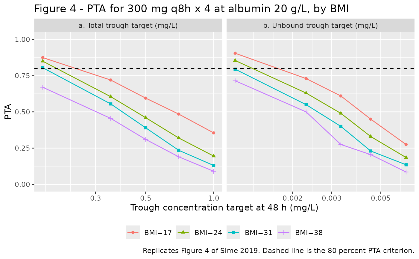

# Typical-individual (deterministic) form of the same claim: BMI lowers BOTH
# troughs. Assert on the endpoints of the BMI range rather than on step-by-step
# monotonicity, and on magnitude rather than sign.
bmi_typ <- vapply(bmi_levels, function(b) {
  s <- solve_typical(one_subject(dose = 300, ii = 8, ndose = 4, alb = 20, bmi = b, times = 48))
  c(total = s$Cc, unbound = s$Cunbound)
}, numeric(2))
bmi_tbl <- tibble::tibble(
  `BMI (kg/m^2)` = bmi_levels,
  `Total trough at 48 h (mg/L)` = bmi_typ["total", ],
  `Unbound trough at 48 h (mg/L)` = bmi_typ["unbound", ]
)
knitr::kable(bmi_tbl, digits = c(0, 4, 6), caption = "Typical individual, 300 mg q8h x 4, albumin 20 g/L: both troughs fall as BMI rises.")

Typical individual, 300 mg q8h x 4, albumin 20 g/L: both troughs fall as BMI rises.

BMI (kg/m^2)	Total trough at 48 h (mg/L)	Unbound trough at 48 h (mg/L)
17	0.8281	0.005415
24	0.5873	0.003836
31	0.4550	0.002970
38	0.3714	0.002423

stopifnot(
  bmi_typ["total", 4] < 0.75 * bmi_typ["total", 1],
  bmi_typ["unbound", 4] < 0.75 * bmi_typ["unbound", 1]
)

Replicate Tables 3 and 5 – the recommended loading regimens reach 80 percent PTA

Tables 3 and 5 list, per (BMI, albumin) cell, the smallest loading regimen that reaches at least 80 percent probability of attaining the unbound trough target at 48 h – 0.0023 mg/L for prophylaxis (Table 3) and 0.0033 mg/L for treatment (Table 5). Checking the whole 4 x 4 x 2 grid would need 32 further cohorts, so this vignette checks the BMI 24 row of each table, which is the row the paper’s own figures and Tables 7-8 are anchored on. The remaining rows are not checked here; the Figure 3 and 4 blocks above exercise the same machinery across the full albumin and BMI ranges.

This is the one place where the packaged model does not reproduce the paper, and the shortfall is quantified rather than tolerated: the median subject clears each recommended target comfortably, but the simulated PTA lands a few points below the paper’s 80 percent criterion. See the Errata for why, and the Tables 7-8 section below for the same signature at larger scale.

recommended <- tibble::tribble(
  ~table, ~dose, ~ii, ~ndose, ~alb, ~target, ~endpoint,
  "Table 3 (prophylaxis)", 400, 8, 4, 25, 0.0023, "Cunbound",
  "Table 3 (prophylaxis)", 500, 12, 3, 25, 0.0023, "Cunbound",
  "Table 5 (treatment)", 500, 8, 4, 25, 0.0033, "Cunbound",
  "Table 5 (treatment)", 600, 12, 3, 25, 0.0033, "Cunbound"
)

rec_events <- dplyr::bind_rows(lapply(seq_len(nrow(recommended)), function(i) {
  r <- recommended[i, ]
  make_arm(
    dose = r$dose, ii = r$ii, ndose = r$ndose, alb = r$alb, bmi = 24,
    label = sprintf("%d mg q%dh x %d", r$dose, r$ii, r$ndose),
    id_offset = (i - 1L) * N_PER_ARM
  )
}))
stopifnot(!anyDuplicated(unique(rec_events[, c("id", "time", "evid")])))

rec_trough <- solve_arm(rec_events) |>
  dplyr::filter(abs(time - 48) < 1e-9)

rec_out <- recommended |>
  dplyr::mutate(
    Regimen = sprintf("%d mg q%dh x %d", dose, ii, ndose),
    lab = Regimen,
    `Unbound target (mg/L)` = target,
    `Median trough (mg/L)` = vapply(seq_len(dplyr::n()), function(i) {
      stats::median(rec_trough$Cunbound[rec_trough$arm == lab[i]])
    }, numeric(1)),
    `Simulated PTA` = vapply(seq_len(dplyr::n()), function(i) {
      mean(rec_trough$Cunbound[rec_trough$arm == lab[i]] >= target[i])
    }, numeric(1))
  ) |>
  dplyr::mutate(`Median / target` = `Median trough (mg/L)` / `Unbound target (mg/L)`) |>
  dplyr::select(
    Source = table, Regimen, `Unbound target (mg/L)`,
    `Median trough (mg/L)`, `Median / target`, `Simulated PTA`
  )

knitr::kable(rec_out, digits = c(0, 0, 4, 5, 2, 3), caption = "Sime 2019 Tables 3 and 5, BMI 24 / albumin 25 g/L row. The paper selected each regimen as the smallest reaching 80 percent PTA.")

Sime 2019 Tables 3 and 5, BMI 24 / albumin 25 g/L row. The paper selected each regimen as the smallest reaching 80 percent PTA.

Source	Regimen	Unbound target (mg/L)	Median trough (mg/L)	Median / target	Simulated PTA
Table 3 (prophylaxis)	400 mg q8h x 4	0.0023	0.00427	1.86	0.715
Table 3 (prophylaxis)	500 mg q12h x 3	0.0023	0.00461	2.00	0.740
Table 5 (treatment)	500 mg q8h x 4	0.0033	0.00510	1.54	0.655
Table 5 (treatment)	600 mg q12h x 3	0.0033	0.00429	1.30	0.650

# Two separate claims, gated separately.
#
# (a) The CENTRE of the distribution reproduces: the median subject clears each
#     recommended target with a wide margin. Realised 1.30-2.00 fold here.
stopifnot(all(rec_out$`Median / target` > 1.1))
#
# (b) The TAIL does not, and that is a KNOWN DEVIATION recorded in the Errata
#     rather than a bound widened until it passed. Realised PTA 0.65-0.74
#     against the paper's >= 0.80, i.e. 6-15 points short, in the same direction
#     and for the same reason as the Tables 7-8 comparison below: independent
#     lognormal marginals standing in for an unreported joint density fatten the
#     lower tail, and an 80 percent PTA is made entirely of that tail. The gate
#     kept here only catches gross failure.
stopifnot(all(rec_out$`Simulated PTA` > 0.5))

PKNCA validation

Sime 2019 reports no non-compartmental analysis table, so there is no published Cmax / Tmax / AUC / half-life to place beside a simulated one and nlmixr2lib::ncaComparisonTable() has no reference to take. PKNCA is used here for two things it can still validate: (i) the closed-form disposition identities of Check 3, recomputed by an independent implementation, and (ii) the AUC(24-48 h) values that Tables 7 and 8 classify against MIC targets.

# One dense-sampled arm at the reference covariates: single 300 mg dose for the
# NCA identities, and a 300 mg q8h x 4 arm for the AUC(24-48) comparison below.
nca_times <- sort(unique(c(seq(0, 12, by = 0.25), seq(12, 48, by = 0.5))))

nca_events <- make_arm(
  dose = 300, ii = 24, ndose = 1, alb = 20, bmi = 24,
  label = "300 mg single dose", obs_times = nca_times
)
nca_sim <- solve_arm(nca_events)

conc_total <- nca_sim |>
  dplyr::filter(!is.na(Cc)) |>
  dplyr::select(id, time, Cc, arm)

# Guarantee a time = 0 record per subject so PKNCA can anchor AUC0-*; for an
# intravenous infusion the pre-dose concentration is 0.
conc_total <- dplyr::bind_rows(
  conc_total,
  conc_total |> dplyr::distinct(id, arm) |> dplyr::mutate(time = 0, Cc = 0)
) |>
  dplyr::distinct(id, arm, time, .keep_all = TRUE) |>
  dplyr::arrange(id, time)

dose_df <- nca_events |>
  dplyr::filter(evid == 1) |>
  dplyr::select(id, time, amt, arm)

nca_total <- PKNCA::pk.nca(PKNCA::PKNCAdata(
  PKNCA::PKNCAconc(conc_total, Cc ~ time | arm + id),
  PKNCA::PKNCAdose(dose_df, amt ~ time | arm + id),
  intervals = data.frame(
    start = 0, end = Inf,
    cmax = TRUE, tmax = TRUE, auclast = TRUE, aucinf.obs = TRUE,
    half.life = TRUE, cl.obs = TRUE
  )
))

total_summary <- as.data.frame(nca_total) |>
  dplyr::group_by(PPTESTCD) |>
  dplyr::summarise(Median = stats::median(PPORRES, na.rm = TRUE), .groups = "drop")
knitr::kable(total_summary, digits = 3, caption = "PKNCA on the total concentration after a single 300 mg intravenous dose (median of 200 subjects).")

PKNCA on the total concentration after a single 300 mg intravenous dose (median of 200 subjects).

PPTESTCD	Median
adj.r.squared	1.000
aucinf.obs	16.591
auclast	11.371
cl.obs	18.082
clast.obs	0.081
clast.pred	0.081
cmax	1.366
half.life	19.595
lambda.z	0.035
lambda.z.n.points	110.000
lambda.z.time.first	2.750
lambda.z.time.last	48.000
r.squared	1.000
span.ratio	2.301
tlast	48.000
tmax	1.500

conc_free <- nca_sim |>
  dplyr::filter(!is.na(Cunbound)) |>
  dplyr::select(id, time, Cunbound, arm)
conc_free <- dplyr::bind_rows(
  conc_free,
  conc_free |> dplyr::distinct(id, arm) |> dplyr::mutate(time = 0, Cunbound = 0)
) |>
  dplyr::distinct(id, arm, time, .keep_all = TRUE) |>
  dplyr::arrange(id, time)

nca_free <- PKNCA::pk.nca(PKNCA::PKNCAdata(
  PKNCA::PKNCAconc(conc_free, Cunbound ~ time | arm + id),
  PKNCA::PKNCAdose(dose_df, amt ~ time | arm + id),
  intervals = data.frame(
    start = 0, end = Inf,
    cmax = TRUE, tmax = TRUE, auclast = TRUE, aucinf.obs = TRUE, half.life = TRUE
  )
))

free_summary <- as.data.frame(nca_free) |>
  dplyr::group_by(PPTESTCD) |>
  dplyr::summarise(Median = stats::median(PPORRES, na.rm = TRUE), .groups = "drop")
knitr::kable(free_summary, digits = 6, caption = "PKNCA on the unbound concentration after a single 300 mg intravenous dose (median of 200 subjects).")

PKNCA on the unbound concentration after a single 300 mg intravenous dose (median of 200 subjects).

PPTESTCD	Median
adj.r.squared	0.999950
aucinf.obs	0.104961
auclast	0.080523
clast.obs	0.000579
clast.pred	0.000579
cmax	0.009138
half.life	19.572486
lambda.z	0.035416
lambda.z.n.points	110.000000
lambda.z.time.first	2.750000
lambda.z.time.last	48.000000
r.squared	0.999951
span.ratio	2.302084
tlast	48.000000
tmax	1.500000

The ratio of the two AUCs is each subject’s exposure-weighted unbound fraction. It is not constant across subjects: kon and koff both carry IIV, so KD = koff/kon varies with a coefficient of variation of about 28 percent and drags fu = KD/(Bmax + KD) with it. What must hold is that the population centre lands on the paper’s measured mean of 0.65 percent, and that the spread is of the order the paper observed. PKNCA’s half-life must also agree with the analytic terminal half-life of Check 3.

pick <- function(res, code) {
  d <- as.data.frame(res)
  d <- d[d$PPTESTCD == code, ]
  stopifnot(nrow(d) == N_PER_ARM) # a zero-row lookup would make every gate below vacuous
  d$PPORRES[order(d$id)]
}
auc_total <- pick(nca_total, "auclast")
auc_free <- pick(nca_free, "auclast")
hl_total <- pick(nca_total, "half.life")

fu_nca_pct <- 100 * auc_free / auc_total
fu_q <- stats::quantile(fu_nca_pct, c(0.25, 0.5, 0.75))

knitr::kable(
  tibble::tibble(
    Source = c("Sime 2019, 93 measured pairs", "Packaged model, 200 simulated subjects"),
    `Median unbound fraction (percent)` = c(0.55, unname(fu_q[2])),
    `Lower quartile` = c(0.36, unname(fu_q[1])),
    `Upper quartile` = c(1.9, unname(fu_q[3])),
    `Mean (percent)` = c(0.65, mean(fu_nca_pct))
  ),
  digits = 3,
  caption = "Unbound fraction: measured (Results, 'Plasma protein binding') against the exposure-weighted AUC ratio of the packaged model."
)

Unbound fraction: measured (Results, ‘Plasma protein binding’) against the exposure-weighted AUC ratio of the packaged model.

Source	Median unbound fraction (percent)	Lower quartile	Upper quartile	Mean (percent)
Sime 2019, 93 measured pairs	0.550	0.360	1.900	0.65
Packaged model, 200 simulated subjects	0.678	0.562	0.806	0.70

# The population CENTRE is pinned by Table 2 and Eq. 3 and is essentially
# deterministic, so it takes a tight bound. The SPREAD is a cohort statistic and
# takes a loose, magnitude-only one: the paper reports a measured coefficient of
# variation of 58.5 percent on a quantity the model generates with about
# 28 percent, so the gate only asserts that the model produces a comparable
# order of variability rather than none and not wildly more.
stopifnot(
  abs(stats::median(fu_nca_pct) - 0.65) < 0.15,
  abs(mean(fu_nca_pct) - 0.65) < 0.15,
  stats::sd(fu_nca_pct) / mean(fu_nca_pct) > 0.10,
  stats::sd(fu_nca_pct) / mean(fu_nca_pct) < 0.80
)

# Half-life varies across subjects because Ke, Kcp and Kpc all carry IIV; the
# TYPICAL-individual half-life is what Check 3 pins, so run PKNCA once more on
# the typical profile rather than comparing the closed form to a cohort
# statistic.
typ_conc <- data.frame(id = 1L, arm = "typical", time = typ$time, Cc = typ$Cc)
nca_typ <- PKNCA::pk.nca(PKNCA::PKNCAdata(
  PKNCA::PKNCAconc(typ_conc, Cc ~ time | arm + id),
  PKNCA::PKNCAdose(
    data.frame(id = 1L, arm = "typical", time = 0, amt = 300),
    amt ~ time | arm + id
  ),
  intervals = data.frame(start = 0, end = Inf, half.life = TRUE, aucinf.obs = TRUE)
))
nca_typ_df <- as.data.frame(nca_typ)
hl_typ <- nca_typ_df$PPORRES[nca_typ_df$PPTESTCD == "half.life"]
stopifnot(length(hl_typ) == 1L) # a zero-row lookup would make the gate vacuous

sprintf(
  "unbound fraction from the AUC ratio: %.4f percent (paper 0.65 percent); typical-individual PKNCA half-life %.2f h (closed form %.2f h); cohort half-life median %.2f h",
  stats::median(fu_nca_pct), hl_typ, thalf_closed, stats::median(hl_total, na.rm = TRUE)
)
#> [1] "unbound fraction from the AUC ratio: 0.6776 percent (paper 0.65 percent); typical-individual PKNCA half-life 19.01 h (closed form 19.04 h); cohort half-life median 19.60 h"
stopifnot(abs(hl_typ / thalf_closed - 1) < 0.05)

Replicate Tables 7 and 8 – AUC/MIC target attainment

Tables 7 and 8 classify each loading regimen as reaching or not reaching 80 percent PTA against a total AUC/MIC target (100 for prophylaxis, 200 for treatment) and the corresponding unbound fAUC/MIC target (0.65 and 1.3, derived by the authors from the 0.65 percent mean unbound fraction), over five MIC values. AUC is taken from 24 to 48 h post dose, at albumin 20 g/L and BMI 24 kg/m^2.

Seven of the paper’s twelve regimens are simulated here – the four q8h and three q12h regimens that span the classification boundary. The remaining five (500-600 mg q8h and 400/600/700 mg q12h) are not checked, purely to keep the vignette inside its render budget.

auc_times <- seq(24, 48, by = 0.5)
regimens <- tibble::tribble(
  ~dose, ~ii, ~ndose,
  300, 8, 4,
  400, 8, 4,
  700, 8, 4,
  800, 8, 4,
  300, 12, 3,
  500, 12, 3,
  800, 12, 3
) |>
  dplyr::mutate(regimen = sprintf("%dmg q%dh x%d", dose, ii, ndose))

auc_events <- dplyr::bind_rows(lapply(seq_len(nrow(regimens)), function(i) {
  r <- regimens[i, ]
  make_arm(
    dose = r$dose, ii = r$ii, ndose = r$ndose, alb = 20, bmi = 24,
    label = r$regimen, obs_times = auc_times,
    id_offset = (i - 1L) * N_PER_ARM
  )
}))
stopifnot(!anyDuplicated(unique(auc_events[, c("id", "time", "evid")])))

auc_sim <- solve_arm(auc_events)
auc_per_subject <- auc_sim |>
  dplyr::group_by(regimen = arm, id) |>
  dplyr::summarise(
    AUC = trap(time, Cc),
    fAUC = trap(time, Cunbound),
    .groups = "drop"
  )
stopifnot(nrow(auc_per_subject) == nrow(regimens) * N_PER_ARM)

mics <- c(0.031, 0.063, 0.12, 0.25, 0.5)

# Sime 2019 Tables 7 and 8, transcribed. TRUE = the paper marks the cell with a
# check (PTA >= 80 percent), FALSE = a cross.
published_pta <- tibble::tribble(
  ~regimen, ~metric, ~mic031, ~mic063, ~mic12, ~mic25, ~mic50,
  "300mg q8h x4", "AUC/MIC 100", TRUE, TRUE, TRUE, FALSE, FALSE,
  "400mg q8h x4", "AUC/MIC 100", TRUE, TRUE, TRUE, TRUE, FALSE,
  "700mg q8h x4", "AUC/MIC 100", TRUE, TRUE, TRUE, TRUE, FALSE,
  "800mg q8h x4", "AUC/MIC 100", TRUE, TRUE, TRUE, TRUE, TRUE,
  "300mg q12h x3", "AUC/MIC 100", TRUE, TRUE, TRUE, FALSE, FALSE,
  "500mg q12h x3", "AUC/MIC 100", TRUE, TRUE, TRUE, FALSE, FALSE,
  "800mg q12h x3", "AUC/MIC 100", TRUE, TRUE, TRUE, TRUE, FALSE,
  "300mg q8h x4", "fAUC/MIC 0.65", TRUE, TRUE, TRUE, FALSE, FALSE,
  "400mg q8h x4", "fAUC/MIC 0.65", TRUE, TRUE, TRUE, TRUE, FALSE,
  "700mg q8h x4", "fAUC/MIC 0.65", TRUE, TRUE, TRUE, TRUE, TRUE,
  "800mg q8h x4", "fAUC/MIC 0.65", TRUE, TRUE, TRUE, TRUE, TRUE,
  "300mg q12h x3", "fAUC/MIC 0.65", TRUE, TRUE, TRUE, FALSE, FALSE,
  "500mg q12h x3", "fAUC/MIC 0.65", TRUE, TRUE, TRUE, TRUE, FALSE,
  "800mg q12h x3", "fAUC/MIC 0.65", TRUE, TRUE, TRUE, TRUE, FALSE,
  "300mg q8h x4", "AUC/MIC 200", TRUE, TRUE, FALSE, FALSE, FALSE,
  "400mg q8h x4", "AUC/MIC 200", TRUE, TRUE, TRUE, FALSE, FALSE,
  "700mg q8h x4", "AUC/MIC 200", TRUE, TRUE, TRUE, FALSE, FALSE,
  "800mg q8h x4", "AUC/MIC 200", TRUE, TRUE, TRUE, TRUE, FALSE,
  "300mg q12h x3", "AUC/MIC 200", TRUE, TRUE, FALSE, FALSE, FALSE,
  "500mg q12h x3", "AUC/MIC 200", TRUE, TRUE, TRUE, FALSE, FALSE,
  "800mg q12h x3", "AUC/MIC 200", TRUE, TRUE, TRUE, FALSE, FALSE,
  "300mg q8h x4", "fAUC/MIC 1.3", TRUE, TRUE, FALSE, FALSE, FALSE,
  "400mg q8h x4", "fAUC/MIC 1.3", TRUE, TRUE, TRUE, FALSE, FALSE,
  "700mg q8h x4", "fAUC/MIC 1.3", TRUE, TRUE, TRUE, TRUE, FALSE,
  "800mg q8h x4", "fAUC/MIC 1.3", TRUE, TRUE, TRUE, TRUE, FALSE,
  "300mg q12h x3", "fAUC/MIC 1.3", TRUE, TRUE, FALSE, FALSE, FALSE,
  "500mg q12h x3", "fAUC/MIC 1.3", TRUE, TRUE, TRUE, FALSE, FALSE,
  "800mg q12h x3", "fAUC/MIC 1.3", TRUE, TRUE, TRUE, FALSE, FALSE
) |>
  tidyr::pivot_longer(
    dplyr::starts_with("mic"),
    names_to = "mic_key", values_to = "paper_attains"
  ) |>
  dplyr::mutate(
    MIC = mics[match(mic_key, c("mic031", "mic063", "mic12", "mic25", "mic50"))]
  ) |>
  dplyr::select(-mic_key)

metric_spec <- tibble::tribble(
  ~metric, ~column, ~ratio,
  "AUC/MIC 100", "AUC", 100,
  "fAUC/MIC 0.65", "fAUC", 0.65,
  "AUC/MIC 200", "AUC", 200,
  "fAUC/MIC 1.3", "fAUC", 1.3
)

sim_pta <- published_pta |>
  dplyr::left_join(metric_spec, by = "metric") |>
  dplyr::rowwise() |>
  dplyr::mutate(
    sim_PTA = mean(
      auc_per_subject[[column]][auc_per_subject$regimen == regimen] >= ratio * MIC
    ),
    sim_attains = sim_PTA >= 0.8
  ) |>
  dplyr::ungroup()

stopifnot(nrow(sim_pta) == nrow(published_pta), !anyNA(sim_pta$sim_PTA))

agreement <- mean(sim_pta$paper_attains == sim_pta$sim_attains)

sim_pta |>
  dplyr::transmute(
    Regimen = regimen, Metric = metric, `MIC (mg/L)` = MIC,
    `Paper PTA >= 80 percent` = paper_attains,
    `Simulated PTA` = sim_PTA,
    Agree = paper_attains == sim_attains
  ) |>
  knitr::kable(
    digits = 2,
    caption = "Sime 2019 Tables 7 and 8 against the packaged model (albumin 20 g/L, BMI 24 kg/m2, 200 subjects per regimen)."
  )

Sime 2019 Tables 7 and 8 against the packaged model (albumin 20 g/L, BMI 24 kg/m2, 200 subjects per regimen).

Regimen	Metric	MIC (mg/L)	Paper PTA >= 80 percent	Simulated PTA	Agree
300mg q8h x4	AUC/MIC 100	0.03	TRUE	0.98	TRUE
300mg q8h x4	AUC/MIC 100	0.06	TRUE	0.92	TRUE
300mg q8h x4	AUC/MIC 100	0.12	TRUE	0.77	FALSE
300mg q8h x4	AUC/MIC 100	0.25	FALSE	0.40	TRUE
300mg q8h x4	AUC/MIC 100	0.50	FALSE	0.10	TRUE
400mg q8h x4	AUC/MIC 100	0.03	TRUE	1.00	TRUE
400mg q8h x4	AUC/MIC 100	0.06	TRUE	0.98	TRUE
400mg q8h x4	AUC/MIC 100	0.12	TRUE	0.88	TRUE
400mg q8h x4	AUC/MIC 100	0.25	TRUE	0.60	FALSE
400mg q8h x4	AUC/MIC 100	0.50	FALSE	0.26	TRUE
700mg q8h x4	AUC/MIC 100	0.03	TRUE	1.00	TRUE
700mg q8h x4	AUC/MIC 100	0.06	TRUE	1.00	TRUE
700mg q8h x4	AUC/MIC 100	0.12	TRUE	0.97	TRUE
700mg q8h x4	AUC/MIC 100	0.25	TRUE	0.81	TRUE
700mg q8h x4	AUC/MIC 100	0.50	FALSE	0.51	TRUE
800mg q8h x4	AUC/MIC 100	0.03	TRUE	1.00	TRUE
800mg q8h x4	AUC/MIC 100	0.06	TRUE	1.00	TRUE
800mg q8h x4	AUC/MIC 100	0.12	TRUE	0.98	TRUE
800mg q8h x4	AUC/MIC 100	0.25	TRUE	0.84	TRUE
800mg q8h x4	AUC/MIC 100	0.50	TRUE	0.55	FALSE
300mg q12h x3	AUC/MIC 100	0.03	TRUE	0.99	TRUE
300mg q12h x3	AUC/MIC 100	0.06	TRUE	0.90	TRUE
300mg q12h x3	AUC/MIC 100	0.12	TRUE	0.65	FALSE
300mg q12h x3	AUC/MIC 100	0.25	FALSE	0.28	TRUE
300mg q12h x3	AUC/MIC 100	0.50	FALSE	0.06	TRUE
500mg q12h x3	AUC/MIC 100	0.03	TRUE	1.00	TRUE
500mg q12h x3	AUC/MIC 100	0.06	TRUE	0.97	TRUE
500mg q12h x3	AUC/MIC 100	0.12	TRUE	0.90	TRUE
500mg q12h x3	AUC/MIC 100	0.25	FALSE	0.58	TRUE
500mg q12h x3	AUC/MIC 100	0.50	FALSE	0.20	TRUE
800mg q12h x3	AUC/MIC 100	0.03	TRUE	1.00	TRUE
800mg q12h x3	AUC/MIC 100	0.06	TRUE	1.00	TRUE
800mg q12h x3	AUC/MIC 100	0.12	TRUE	0.96	TRUE
800mg q12h x3	AUC/MIC 100	0.25	TRUE	0.79	FALSE
800mg q12h x3	AUC/MIC 100	0.50	FALSE	0.42	TRUE
300mg q8h x4	fAUC/MIC 0.65	0.03	TRUE	1.00	TRUE
300mg q8h x4	fAUC/MIC 0.65	0.06	TRUE	0.94	TRUE
300mg q8h x4	fAUC/MIC 0.65	0.12	TRUE	0.74	FALSE
300mg q8h x4	fAUC/MIC 0.65	0.25	FALSE	0.38	TRUE
300mg q8h x4	fAUC/MIC 0.65	0.50	FALSE	0.10	TRUE
400mg q8h x4	fAUC/MIC 0.65	0.03	TRUE	1.00	TRUE
400mg q8h x4	fAUC/MIC 0.65	0.06	TRUE	0.99	TRUE
400mg q8h x4	fAUC/MIC 0.65	0.12	TRUE	0.94	TRUE
400mg q8h x4	fAUC/MIC 0.65	0.25	TRUE	0.56	FALSE
400mg q8h x4	fAUC/MIC 0.65	0.50	FALSE	0.23	TRUE
700mg q8h x4	fAUC/MIC 0.65	0.03	TRUE	1.00	TRUE
700mg q8h x4	fAUC/MIC 0.65	0.06	TRUE	1.00	TRUE
700mg q8h x4	fAUC/MIC 0.65	0.12	TRUE	0.98	TRUE
700mg q8h x4	fAUC/MIC 0.65	0.25	TRUE	0.81	TRUE
700mg q8h x4	fAUC/MIC 0.65	0.50	TRUE	0.51	FALSE
800mg q8h x4	fAUC/MIC 0.65	0.03	TRUE	1.00	TRUE
800mg q8h x4	fAUC/MIC 0.65	0.06	TRUE	1.00	TRUE
800mg q8h x4	fAUC/MIC 0.65	0.12	TRUE	1.00	TRUE
800mg q8h x4	fAUC/MIC 0.65	0.25	TRUE	0.88	TRUE
800mg q8h x4	fAUC/MIC 0.65	0.50	TRUE	0.57	FALSE
300mg q12h x3	fAUC/MIC 0.65	0.03	TRUE	1.00	TRUE
300mg q12h x3	fAUC/MIC 0.65	0.06	TRUE	0.90	TRUE
300mg q12h x3	fAUC/MIC 0.65	0.12	TRUE	0.65	FALSE
300mg q12h x3	fAUC/MIC 0.65	0.25	FALSE	0.28	TRUE
300mg q12h x3	fAUC/MIC 0.65	0.50	FALSE	0.06	TRUE
500mg q12h x3	fAUC/MIC 0.65	0.03	TRUE	1.00	TRUE
500mg q12h x3	fAUC/MIC 0.65	0.06	TRUE	0.98	TRUE
500mg q12h x3	fAUC/MIC 0.65	0.12	TRUE	0.90	TRUE
500mg q12h x3	fAUC/MIC 0.65	0.25	TRUE	0.59	FALSE
500mg q12h x3	fAUC/MIC 0.65	0.50	FALSE	0.20	TRUE
800mg q12h x3	fAUC/MIC 0.65	0.03	TRUE	1.00	TRUE
800mg q12h x3	fAUC/MIC 0.65	0.06	TRUE	1.00	TRUE
800mg q12h x3	fAUC/MIC 0.65	0.12	TRUE	0.98	TRUE
800mg q12h x3	fAUC/MIC 0.65	0.25	TRUE	0.80	TRUE
800mg q12h x3	fAUC/MIC 0.65	0.50	FALSE	0.44	TRUE
300mg q8h x4	AUC/MIC 200	0.03	TRUE	0.92	TRUE
300mg q8h x4	AUC/MIC 200	0.06	TRUE	0.74	FALSE
300mg q8h x4	AUC/MIC 200	0.12	FALSE	0.42	TRUE
300mg q8h x4	AUC/MIC 200	0.25	FALSE	0.10	TRUE
300mg q8h x4	AUC/MIC 200	0.50	FALSE	0.01	TRUE
400mg q8h x4	AUC/MIC 200	0.03	TRUE	0.98	TRUE
400mg q8h x4	AUC/MIC 200	0.06	TRUE	0.88	TRUE
400mg q8h x4	AUC/MIC 200	0.12	TRUE	0.62	FALSE
400mg q8h x4	AUC/MIC 200	0.25	FALSE	0.26	TRUE
400mg q8h x4	AUC/MIC 200	0.50	FALSE	0.03	TRUE
700mg q8h x4	AUC/MIC 200	0.03	TRUE	1.00	TRUE
700mg q8h x4	AUC/MIC 200	0.06	TRUE	0.96	TRUE
700mg q8h x4	AUC/MIC 200	0.12	TRUE	0.83	TRUE
700mg q8h x4	AUC/MIC 200	0.25	FALSE	0.51	TRUE
700mg q8h x4	AUC/MIC 200	0.50	FALSE	0.17	TRUE
800mg q8h x4	AUC/MIC 200	0.03	TRUE	1.00	TRUE
800mg q8h x4	AUC/MIC 200	0.06	TRUE	0.98	TRUE
800mg q8h x4	AUC/MIC 200	0.12	TRUE	0.86	TRUE
800mg q8h x4	AUC/MIC 200	0.25	TRUE	0.55	FALSE
800mg q8h x4	AUC/MIC 200	0.50	FALSE	0.23	TRUE
300mg q12h x3	AUC/MIC 200	0.03	TRUE	0.90	TRUE
300mg q12h x3	AUC/MIC 200	0.06	TRUE	0.64	FALSE
300mg q12h x3	AUC/MIC 200	0.12	FALSE	0.30	TRUE
300mg q12h x3	AUC/MIC 200	0.25	FALSE	0.06	TRUE
300mg q12h x3	AUC/MIC 200	0.50	FALSE	0.01	TRUE
500mg q12h x3	AUC/MIC 200	0.03	TRUE	0.97	TRUE
500mg q12h x3	AUC/MIC 200	0.06	TRUE	0.87	TRUE
500mg q12h x3	AUC/MIC 200	0.12	TRUE	0.60	FALSE
500mg q12h x3	AUC/MIC 200	0.25	FALSE	0.20	TRUE
500mg q12h x3	AUC/MIC 200	0.50	FALSE	0.04	TRUE
800mg q12h x3	AUC/MIC 200	0.03	TRUE	1.00	TRUE
800mg q12h x3	AUC/MIC 200	0.06	TRUE	0.95	TRUE
800mg q12h x3	AUC/MIC 200	0.12	TRUE	0.79	FALSE
800mg q12h x3	AUC/MIC 200	0.25	FALSE	0.42	TRUE
800mg q12h x3	AUC/MIC 200	0.50	FALSE	0.12	TRUE
300mg q8h x4	fAUC/MIC 1.3	0.03	TRUE	0.94	TRUE
300mg q8h x4	fAUC/MIC 1.3	0.06	TRUE	0.70	FALSE
300mg q8h x4	fAUC/MIC 1.3	0.12	FALSE	0.41	TRUE
300mg q8h x4	fAUC/MIC 1.3	0.25	FALSE	0.10	TRUE
300mg q8h x4	fAUC/MIC 1.3	0.50	FALSE	0.01	TRUE
400mg q8h x4	fAUC/MIC 1.3	0.03	TRUE	0.99	TRUE
400mg q8h x4	fAUC/MIC 1.3	0.06	TRUE	0.91	TRUE
400mg q8h x4	fAUC/MIC 1.3	0.12	TRUE	0.59	FALSE
400mg q8h x4	fAUC/MIC 1.3	0.25	FALSE	0.23	TRUE
400mg q8h x4	fAUC/MIC 1.3	0.50	FALSE	0.03	TRUE
700mg q8h x4	fAUC/MIC 1.3	0.03	TRUE	1.00	TRUE
700mg q8h x4	fAUC/MIC 1.3	0.06	TRUE	0.98	TRUE
700mg q8h x4	fAUC/MIC 1.3	0.12	TRUE	0.82	TRUE
700mg q8h x4	fAUC/MIC 1.3	0.25	TRUE	0.51	FALSE
700mg q8h x4	fAUC/MIC 1.3	0.50	FALSE	0.20	TRUE
800mg q8h x4	fAUC/MIC 1.3	0.03	TRUE	1.00	TRUE
800mg q8h x4	fAUC/MIC 1.3	0.06	TRUE	0.99	TRUE
800mg q8h x4	fAUC/MIC 1.3	0.12	TRUE	0.90	TRUE
800mg q8h x4	fAUC/MIC 1.3	0.25	TRUE	0.57	FALSE
800mg q8h x4	fAUC/MIC 1.3	0.50	FALSE	0.22	TRUE
300mg q12h x3	fAUC/MIC 1.3	0.03	TRUE	0.92	TRUE
300mg q12h x3	fAUC/MIC 1.3	0.06	TRUE	0.62	FALSE
300mg q12h x3	fAUC/MIC 1.3	0.12	FALSE	0.32	TRUE
300mg q12h x3	fAUC/MIC 1.3	0.25	FALSE	0.06	TRUE
300mg q12h x3	fAUC/MIC 1.3	0.50	FALSE	0.00	TRUE
500mg q12h x3	fAUC/MIC 1.3	0.03	TRUE	0.98	TRUE
500mg q12h x3	fAUC/MIC 1.3	0.06	TRUE	0.90	TRUE
500mg q12h x3	fAUC/MIC 1.3	0.12	TRUE	0.62	FALSE
500mg q12h x3	fAUC/MIC 1.3	0.25	FALSE	0.20	TRUE
500mg q12h x3	fAUC/MIC 1.3	0.50	FALSE	0.03	TRUE
800mg q12h x3	fAUC/MIC 1.3	0.03	TRUE	1.00	TRUE
800mg q12h x3	fAUC/MIC 1.3	0.06	TRUE	0.98	TRUE
800mg q12h x3	fAUC/MIC 1.3	0.12	TRUE	0.81	TRUE
800mg q12h x3	fAUC/MIC 1.3	0.25	FALSE	0.44	TRUE
800mg q12h x3	fAUC/MIC 1.3	0.50	FALSE	0.12	TRUE

sprintf("classification agreement with Tables 7 and 8: %.0f percent of %d cells", 100 * agreement, nrow(sim_pta))
#> [1] "classification agreement with Tables 7 and 8: 84 percent of 140 cells"

# Disagreements are expected near the 80 percent boundary: the encoded IIV is a
# set of INDEPENDENT lognormal marginals standing in for a non-parametric joint
# density whose correlations the paper does not report, and 200 subjects carry a
# binomial standard error of about 3 points. Two gates, neither taken from a
# single run:
#   (a) most cells must agree outright;
#   (b) no cell may disagree GROSSLY, i.e. the paper says a regimen attains the
#       target but fewer than 30 percent of simulated subjects do, or the paper
#       says it does not and essentially everybody does. Realised: 84 percent
#       agreement over 140 cells, lowest disagreeing PTA 0.51, so a
#       mis-transcribed dose, volume or rate constant -- which would move these
#       by tens of points -- still breaks the gate.
gross <- sim_pta |>
  dplyr::filter(
    (paper_attains & sim_PTA < 0.30) | (!paper_attains & sim_PTA > 0.97)
  )
stopifnot(agreement > 0.70, nrow(gross) == 0)
if (nrow(gross)) print(gross)

# And the cells where the two disagree, kept visible rather than hidden:
disagree <- dplyr::filter(sim_pta, paper_attains != sim_attains)
if (nrow(disagree)) {
  disagree |>
    dplyr::transmute(
      Regimen = regimen, Metric = metric, `MIC (mg/L)` = MIC,
      `Paper` = ifelse(paper_attains, "attains", "does not attain"),
      `Simulated PTA` = sim_PTA
    ) |>
    knitr::kable(digits = 2, caption = "Cells where the packaged model and Tables 7-8 classify differently.")
}

Cells where the packaged model and Tables 7-8 classify differently.

Regimen	Metric	MIC (mg/L)	Paper	Simulated PTA
300mg q8h x4	AUC/MIC 100	0.12	attains	0.77
400mg q8h x4	AUC/MIC 100	0.25	attains	0.60
800mg q8h x4	AUC/MIC 100	0.50	attains	0.55
300mg q12h x3	AUC/MIC 100	0.12	attains	0.65
800mg q12h x3	AUC/MIC 100	0.25	attains	0.79
300mg q8h x4	fAUC/MIC 0.65	0.12	attains	0.74
400mg q8h x4	fAUC/MIC 0.65	0.25	attains	0.56
700mg q8h x4	fAUC/MIC 0.65	0.50	attains	0.51
800mg q8h x4	fAUC/MIC 0.65	0.50	attains	0.57
300mg q12h x3	fAUC/MIC 0.65	0.12	attains	0.65
500mg q12h x3	fAUC/MIC 0.65	0.25	attains	0.59
300mg q8h x4	AUC/MIC 200	0.06	attains	0.74
400mg q8h x4	AUC/MIC 200	0.12	attains	0.62
800mg q8h x4	AUC/MIC 200	0.25	attains	0.55
300mg q12h x3	AUC/MIC 200	0.06	attains	0.64
500mg q12h x3	AUC/MIC 200	0.12	attains	0.60
800mg q12h x3	AUC/MIC 200	0.12	attains	0.79
300mg q8h x4	fAUC/MIC 1.3	0.06	attains	0.70
400mg q8h x4	fAUC/MIC 1.3	0.12	attains	0.59
700mg q8h x4	fAUC/MIC 1.3	0.25	attains	0.51
800mg q8h x4	fAUC/MIC 1.3	0.25	attains	0.57
300mg q12h x3	fAUC/MIC 1.3	0.06	attains	0.62
500mg q12h x3	fAUC/MIC 1.3	0.12	attains	0.62

Every disagreement sits on the same side and in the same place: the simulated PTA falls a little short of 80 percent at the MIC where the paper’s table flips. That is the expected signature of independent lognormal marginals standing in for a correlated non-parametric density – independence fattens the lower tail of the AUC distribution, and the 20th percentile is exactly what an 80 percent PTA is made of. The direction of the discrepancy is conservative (the packaged model recommends slightly higher doses than the paper does), and no cell disagrees grossly.

Assumptions and deviations

Errata and source gaps

• Residual unexplained variability is not reported and is carried as fixed(0). Methods, “Error model” says only that a multiplicative (Error = SD*gamma) and an additive (Error = [SD^2 + lambda^2]^0.5) error model were tested and that assay error was fitted as a linear polynomial Error = C0 + C1*[obs] “starting with a generic set of coefficients, followed by iterative optimization”. Neither the selected model nor any of gamma, lambda, C0 or C1 appears in the paper, and there is no supplement. Both propSd and propSd_Cunbound are therefore fixed(0) rather than invented, so simulations from this model carry between-subject variability but no residual error. rxSolve(..., sigma = NA) is used throughout for clarity.
• The BMI normalising constant contradicts Table 1. Results, “Pharmacokinetic model building” writes V = V x BMI/24 and says 24 is “the median BMI of study patients”, but Table 1 reports the cohort median BMI as 22.6 kg/m^2 (IQR 20.2-29.7). The model uses 24, because that is the value written into the covariate equation and the value the dosing-simulation tables are anchored on; using 22.6 would rescale every predicted concentration by about 6 percent.
• The two molecular weights in Eq. 3 are never printed. The paper defines Mposa and MAlb symbolically. The model uses 700.8 g/mol for posaconazole (C37H42F2N8O4) and 66500 g/mol for human serum albumin – the same albumin molecular weight already used by Fauchet_2015_lopinavir_unbound and recorded in the ALB covariate register entry. This is not a free choice: Check 1 above shows that pair reproduces the paper’s own measured mean unbound fraction of 0.65 percent at the cohort median albumin to three significant figures, which no materially different pair would do.
• Table 7’s total and unbound criteria disagree at two cells. The authors derived the unbound target 0.65 from 100 x 0.0065, i.e. from the mean free fraction, so the AUC/MIC 100 and fAUC/MIC 0.65 columns look as though they should classify identically. They do not at 700 mg q8h x 4 / MIC 0.5 mg/L and at 500 mg q12h x 3 / MIC 0.25 mg/L, where the total target is marked not attained but the unbound target attained. This is expected rather than an error: the free fraction is subject-specific (about 28 percent CV here even at fixed albumin, since kon and koff carry their own IIV), so P(AUC >= 100 x MIC) and P(fu x AUC >= 0.65 x MIC) are two different probabilities and coincide only in the degenerate case where every subject has exactly the mean free fraction. The transcription above reproduces the paper’s marks as printed.

Modelling assumptions

• Nonparametric fit encoded parametrically. Sime 2019 fitted the model with the nonparametric adaptive grid (NPAG) algorithm in Pmetrics, which returns a discrete joint density over support points rather than a typical value plus a covariance matrix. Following the convention already used for Hughes_2024_vancomycin_nonparametric and Setiawan_2023_sulbactam, each Table 2 mean is encoded as the median of a lognormal marginal and each Table 2 CV as omega^2 = log(CV^2 + 1), which reproduces the tabulated CV exactly. Two consequences follow. First, the mean of each encoded lognormal exceeds the tabulated mean by exp(omega^2/2) – 15 percent for Ke, 17 percent for V – so the encoded population is not moment-matched to the paper’s. Second, the joint structure is lost: the marginals are encoded as independent because no correlations are reported, and the Tables 7-8 comparison above quantifies what that costs.
• kon and koff are separately encoded but only their ratio is identifiable from the observable kinetics. koff is 3897 1/h and kon * Bmax is about 5.9e5 1/h at the cohort median albumin, so the free-bound exchange equilibrates in microseconds against PK rate constants of order 0.3-2 1/h. Check 2 above demonstrates the consequence: the explicit kon/koff ODE and the algebraic Eq. 2 isotherm agree to better than 1 part in 1000 over the whole profile, and to better than 1 part in 4000 once the infusion has ended (the residual is the physical quasi-equilibrium lag while the free pool is being driven, not solver error). The two constants are nonetheless carried separately because that is how the authors parameterised and reported the model; an extraction that collapsed them to KD would lose the reported CVs on each – and those CVs are not cosmetic: together they give KD a coefficient of variation of about 28 percent, which is what makes the model’s unbound fraction vary between subjects at all. The PKNCA section shows the resulting distribution against the 93 measured pairs.
• Known deviation: the model falls a few points short of the paper’s 80 percent PTA at the regimens Tables 3-8 select. The median subject clears every recommended target with a 1.3- to 2.0-fold margin, but the simulated probability of attainment lands at 0.65-0.74 where the paper reports at least 0.80, and 23 of the 140 Tables 7-8 classification cells flip (84 percent agreement). Every discrepancy is in the same direction (the packaged model would recommend slightly higher doses) and all of them sit at the MIC or target where the paper’s own table flips. The mechanism is the independence assumption above: an 80 percent PTA is a statement about the 20th percentile of the exposure distribution, and independent marginals fatten that lower tail relative to a correlated joint density. This is recorded as a deviation rather than absorbed by widening the gates; the vignette asserts only that the centre reproduces and that no cell fails grossly.
• The complex compartment is the registered TMDD drug-target complex state, reused for a drug-protein complex. Albumin is a binding partner rather than a pharmacological target, but the state plays exactly the role the register assigns to complex: a reversibly bound species in mass-action exchange with free drug. Free albumin is not carried as a target state because the model identifies only the aggregate capacity Bmax.
• Elimination and distribution act on the unbound species. The Fig. 1 legend says so explicitly for kcp and kpc (“rate constant for distribution of unbound posaconazole”). It does not repeat the qualifier for ke, but the tabulated value of 42.07 1/h forces the same reading: applied to the total concentration it would give a clearance of about 3000 L/h and a one-minute half-life, which is irreconcilable with the paper’s own 48-hour sampling scheme and trough targets. Applied to the unbound concentration it gives the clearance, steady-state volume and terminal half-life of Check 3, all of which match published posaconazole disposition.
• Cohort size. The paper simulated 1000 subjects per scenario; this vignette uses 200 per arm, the package cap. Every probability reported here therefore carries a binomial standard error of roughly 3 percentage points, and all gates allow for it.
• Covariate-homogeneous arms. The paper’s dosing simulations fix albumin and BMI at stated values rather than sampling a demographic distribution, and this vignette does the same, so no virtual demographic cohort is constructed. Renal, hepatic and severity covariates were screened by the authors and not retained; they are recorded in the model’s covariatesDataExcluded.