Fluconazole (Wade 2008)
Source:vignettes/articles/Wade_2008_fluconazole.Rmd
Wade_2008_fluconazole.RmdModel and source
- Citation: Wade KC, Wu D, Kaufman DA, Ward RM, Benjamin DK Jr, Sullivan JE, Ramey N, Jayaraman B, Hoppu K, Adamson PC, Gastonguay MR, Barrett JS. Population pharmacokinetics of fluconazole in young infants. Antimicrob Agents Chemother. 2008. doi:10.1128/AAC.00569-08
- Description: One-compartment intravenous population PK model for fluconazole in preterm and term infants (gestational age 23-40 weeks, postnatal age <120 days) with allometric body weight on CL and V (fixed exponents 0.75 and 1.0, reference 1 kg), power effects of gestational age at birth (reference 26 weeks) and postnatal age (reference 2 weeks) on CL, and an on/off power effect of serum creatinine on CL gated when SCR > 1 mg/dL (Wade 2008).
- Article: https://doi.org/10.1128/AAC.00569-08
Population
Wade et al. (2008) developed a one-compartment population PK model of intravenous fluconazole in 55 preterm and term infants enrolled across two NICHD Pediatric Pharmacology Research Unit (PPRU) studies. Infants were less than 120 days old, ranged in gestational age at birth (BGA) from 23 to 40 weeks (median 26 weeks), and ranged in body weight from 0.451 to 7.125 kg (median 1.020 kg). Postnatal age (PNA) at enrolment was 1 to 88 days (median 16 days). The cohort was 56% male and approximately 50% Caucasian, 40% Black, 10% other race, with 9% reporting Hispanic ethnicity (Wade 2008 Table 1).
Dosing was determined by routine clinical practice and ranged from 3 to 12 mg/kg/dose. The final dataset contained 357 plasma fluconazole observations (217 prospectively timed, 140 scavenged from discarded clinical specimens), with a median of 6.5 samples per infant.
The same metadata is available programmatically via
readModelDb("Wade_2008_fluconazole")()$population.
Source trace
Per-parameter origin is recorded inline next to each
ini() entry in
inst/modeldb/specificDrugs/Wade_2008_fluconazole.R. The
table below collects them in one place for review.
| Equation / parameter | Value | Source location |
|---|---|---|
lcl (CL, L/h) at 1 kg, 26 weeks BGA, 2 weeks PNA,
normal renal function |
log(0.015) |
Wade 2008 Table 3: theta_CL = 0.015 L/h (RSE 5.9%) |
lvc (V, L) at 1 kg |
log(1.024) |
Wade 2008 Table 3: theta_V = 1.024 L (RSE 3.8%) |
e_wt_cl (allometric exponent on CL) |
0.75 (fixed) |
Wade 2008 Table 2: CL base model row,
CL = theta_CL * (wt)^0.75
|
e_wt_vc (allometric exponent on V) |
1.0 (fixed) |
Wade 2008 Table 2: base model row,
V = theta_V * (wt)^1
|
e_ga_cl (exponent on (GA/26)) |
1.739 |
Wade 2008 Table 3: theta_CL-BGA = 1.739 (RSE 18%) |
e_pna_cl (exponent on (PNA/2 weeks)) |
0.237 |
Wade 2008 Table 3: theta_CL-PNA = 0.237 (RSE 24%) |
e_creat_cl (exponent on SCRT for CL when CR = 1) |
-4.896 |
Wade 2008 Table 3: theta_CL-SCRT = -4.896 (RSE 22%) |
CR (renal-impairment switch derived inside model) |
(CREAT > 1) * 1 |
Wade 2008 Methods: dichotomous renal indicator, CR = 1 when measured SCR > 1 mg/dL, else 0 |
etalcl + etalvc ~ c(0.11, 0.014, 0.057) |
variance block | Wade 2008 Table 3: omega^2(CL) = 0.11, omega^2(V) = 0.057, cov(CL,V) = 0.014 |
propSd (proportional residual SD) |
0.1643 |
Wade 2008 Table 3 Sigma 1 (prospective PK) = 0.027 variance -> SD = sqrt(0.027) |
addSd (additive residual SD, ug/mL) |
0.2 |
Wade 2008 Table 3 Sigma 2 (prospective PK) = 0.04 variance -> SD = sqrt(0.04) |
| Eq. for CL | n/a | Wade 2008 abstract:
CL = theta_CL * (wt/1)^0.75 * (BGA/26)^theta_CL-BGA * (PNA/2)^theta_CL-PNA * SCRT^(theta_CL-SCRT * CR)
|
| Eq. for V | n/a | Wade 2008 abstract: V = theta_V * (wt/1)^1
|
Virtual cohort
Wade 2008 study data are not publicly available. Simulations below use a virtual cohort constructed to match the BGA / PNA strata that Wade 2008 Discussion uses to summarise Bayesian individual estimates: typical 24-, 28-, and 32-week-gestation infants. Each stratum is anchored at the typical baseline body weights given in Wade 2008 Discussion (600 g, 1000 g, 1500 g respectively). Serum creatinine is held at 1.0 mg/dL (so CR = 0, no renal impairment) for the maturation-trajectory simulation; the SCR effect is illustrated separately at the end of the vignette.
set.seed(2008)

strata <- tibble(
  stratum = c("BGA 24 wk", "BGA 28 wk", "BGA 32 wk"),
  GA      = c(24, 28, 32),
  WT      = c(0.6, 1.0, 1.5),
  CREAT   = 1.0
)

# Wade 2008 dose-exposure simulation (Figure 4 panels A and B):
# 12 mg/kg/day fluconazole administered for 14 days, dose given as a
# 0.5-h IV infusion once daily.
DOSE_MG_PER_KG <- 12
T_INF          <- 0.5
N_DOSES        <- 14
DOSE_INTERVAL  <- 24
DURATION_H     <- N_DOSES * DOSE_INTERVAL

# Per-subject PNA at first dose: paper enrolled infants from PNA day 1
# upward. Start each virtual infant at PNA = 1 day so the typical
# trajectory matches the paper's day-of-life axis (Figure 4 A/B).
PNA_AT_FIRST_DOSE_DAYS <- 1

n_per_stratum <- 200

make_subject <- function(id, stratum, GA, WT, CREAT, id_offset = 0L) {
  dose_mg <- DOSE_MG_PER_KG * WT
  ev <- rxode2::et(
    amt  = dose_mg,
    rate = dose_mg / T_INF,
    cmt  = "central",
    ii   = DOSE_INTERVAL,
    addl = N_DOSES - 1L,
    time = 0
  )
  obs_grid <- seq(0, DURATION_H, by = 1)
  ev <- rxode2::et(ev, obs_grid)
  df <- as.data.frame(ev)
  df$WT      <- WT
  df$GA      <- GA
  df$CREAT   <- CREAT
  df$stratum <- stratum
  df$id      <- id_offset + id
  # PNA in canonical months, growing in time (1 hour = 1/(24*30.4375) months)
  df$PNA <- (PNA_AT_FIRST_DOSE_DAYS + df$time / 24) / 30.4375
  df
}

events <- bind_rows(lapply(seq_len(nrow(strata)), function(i) {
  s <- strata[i, ]
  bind_rows(lapply(seq_len(n_per_stratum), function(j) {
    make_subject(
      id        = j,
      stratum   = s$stratum,
      GA        = s$GA,
      WT        = s$WT,
      CREAT     = s$CREAT,
      id_offset = (i - 1L) * n_per_stratum
    )
  }))
}))
Simulation
mod <- readModelDb("Wade_2008_fluconazole")()

sim <- rxode2::rxSolve(
  mod,
  events = events,
  keep   = c("stratum", "WT", "GA", "PNA", "CREAT")
) |> as.data.frame()

# Typical-patient profile (zero IIV) for overlay
mod_typ <- rxode2::zeroRe(mod)
sim_typ <- rxode2::rxSolve(
  mod_typ,
  events = events |>
    filter(id %in% c(1L, n_per_stratum + 1L, 2L * n_per_stratum + 1L)),
  keep   = c("stratum", "WT", "GA", "PNA", "CREAT")
) |> as.data.frame()
#> ℹ omega/sigma items treated as zero: 'etalcl', 'etalvc'
#> Warning: multi-subject simulation without without 'omega'
Replicate published results
Figure 4 – AUC24 trajectory by BGA stratum over 14 days of 12 mg/kg/day
Wade 2008 Figure 4 panels A and B show the simulated AUC over each 24-hour dosing interval, stratified by BGA (panel A: 23-29 wk, panel B: 30-40 wk), with the AUC target of 800 mgh/L marked. The replicate below splits the three typical-infant strata (24 / 28 / 32 wk BGA) and overlays the same 800 mgh/L target.
auc24 <- sim |>
  filter(!is.na(Cc)) |>
  mutate(day = floor(time / DOSE_INTERVAL) + 1L) |>
  filter(day <= N_DOSES) |>
  group_by(stratum, id, day) |>
  arrange(time, .by_group = TRUE) |>
  summarise(
    auc24 = PKNCA::pk.calc.auc(conc = Cc, time = time,
                               interval = c(min(time), max(time)),
                               method = "lin up/log down"),
    .groups = "drop"
  )

auc_summary <- auc24 |>
  group_by(stratum, day) |>
  summarise(
    Q10 = quantile(auc24, 0.10, na.rm = TRUE),
    Q50 = quantile(auc24, 0.50, na.rm = TRUE),
    Q90 = quantile(auc24, 0.90, na.rm = TRUE),
    .groups = "drop"
  )

ggplot(auc_summary, aes(day, Q50, colour = stratum, fill = stratum)) +
  geom_ribbon(aes(ymin = Q10, ymax = Q90), alpha = 0.20, colour = NA) +
  geom_line(linewidth = 0.8) +
  geom_hline(yintercept = 800, linetype = "dashed", colour = "grey30") +
  scale_x_continuous(breaks = seq(1, N_DOSES, by = 2)) +
  labs(
    x       = "Day of therapy",
    y       = "Interval AUC over 24 h (mg*h/L)",
    colour  = "Stratum",
    fill    = "Stratum",
    title   = "Figure 4 replicate -- AUC24 over 14 days of 12 mg/kg/day fluconazole",
    caption = paste(
      "Replicates Wade 2008 Figure 4 panels A/B for typical 24/28/32 wk BGA infants.",
      "Ribbon: simulated 10th-90th percentile across N = 200 per stratum.",
      "Dashed line: 800 mg*h/L AUC target."
    )
  ) +
  theme_minimal()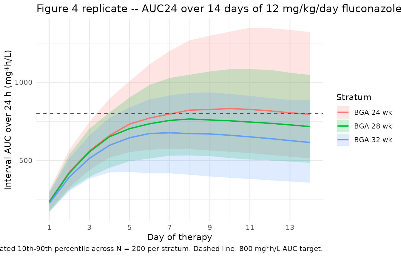
Typical-patient plasma concentration profile
ggplot(sim_typ |> filter(!is.na(Cc)),
       aes(time / 24, Cc, colour = stratum)) +
  geom_line(linewidth = 0.9) +
  scale_x_continuous(breaks = seq(0, 14, by = 2)) +
  labs(
    x       = "Day of therapy",
    y       = "Fluconazole plasma concentration (ug/mL)",
    colour  = "Stratum",
    title   = "Typical-patient fluconazole PK at 12 mg/kg/day IV",
    caption = paste(
      "Wade 2008 dosing assumption: 12 mg/kg fluconazole once daily,",
      "0.5-h IV infusion, 14 doses. Serum creatinine 1.0 mg/dL (CR = 0)."
    )
  ) +
  theme_minimal()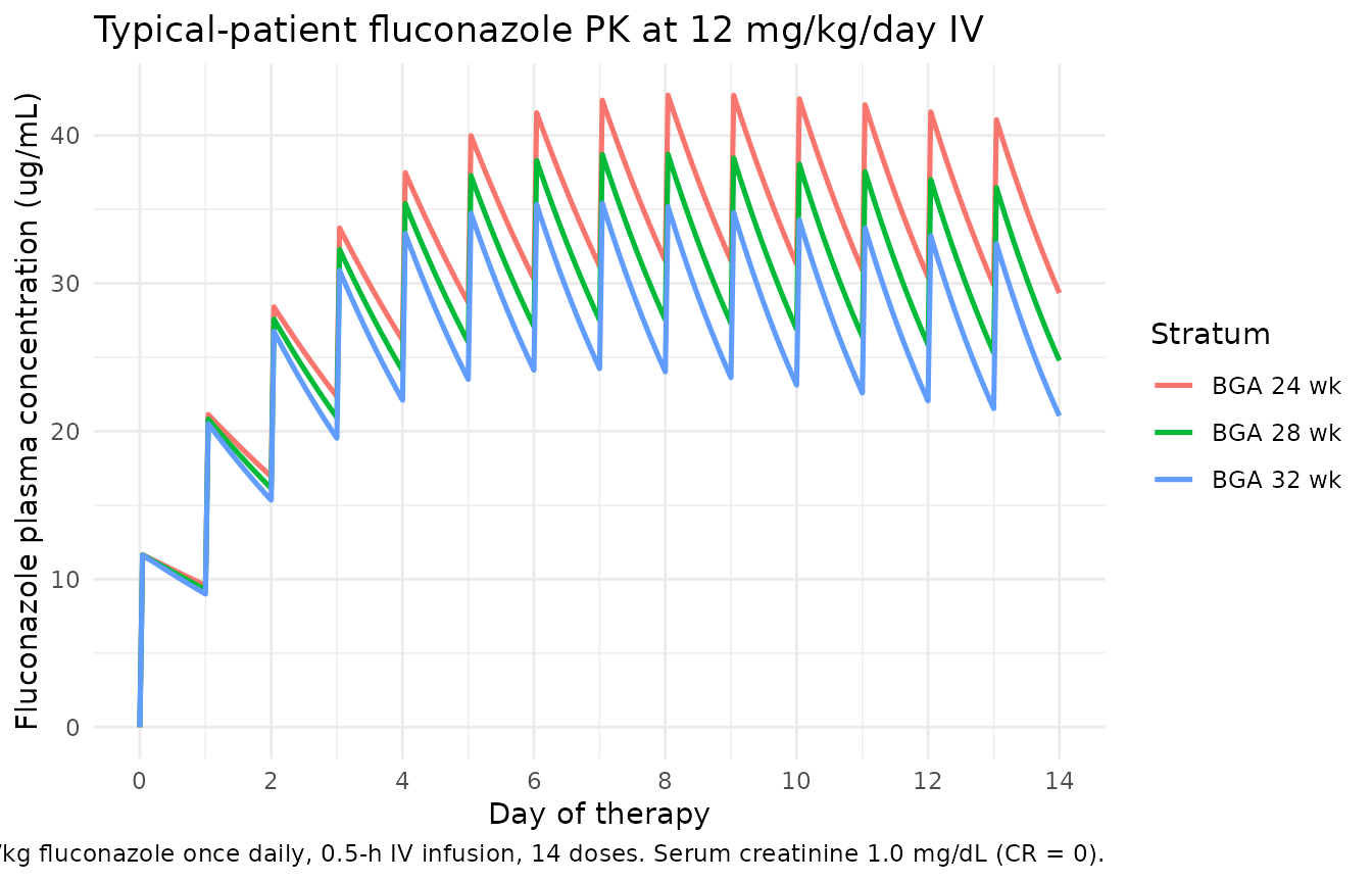
PKNCA validation
Single-dose NCA over the first 24-hour dosing interval, stratified by BGA. The simulated typical-patient CL per kg can be compared against Wade 2008 Discussion: “CL is low at birth: 8, 9, and 10 mL/kg/h for these typical 24-, 28-, and 32-week-gestation infants, respectively.”
sim_nca_single <- sim |>
  filter(time <= DOSE_INTERVAL, !is.na(Cc), Cc > 0) |>
  select(id, time, Cc, stratum)

dose_df_single <- events |>
  filter(evid == 1L, time == 0) |>
  group_by(id) |>
  slice(1) |>
  ungroup() |>
  select(id, time, amt, stratum)

conc_obj_single <- PKNCA::PKNCAconc(sim_nca_single, Cc ~ time | stratum + id)
dose_obj_single <- PKNCA::PKNCAdose(dose_df_single, amt ~ time | stratum + id,
                                    route = "intravascular")

intervals_single <- data.frame(
  start     = 0,
  end       = DOSE_INTERVAL,
  cmax      = TRUE,
  tmax      = TRUE,
  auclast   = TRUE,
  half.life = TRUE
)

nca_data_single <- PKNCA::PKNCAdata(conc_obj_single, dose_obj_single,
                                    intervals = intervals_single)
nca_res_single  <- suppressWarnings(PKNCA::pk.nca(nca_data_single))
nca_df_single   <- as.data.frame(nca_res_single$result)

nca_summary_single <- nca_df_single |>
  group_by(stratum, PPTESTCD) |>
  summarise(
    median = round(median(PPORRES, na.rm = TRUE), 3),
    p05    = round(quantile(PPORRES, 0.05, na.rm = TRUE), 3),
    p95    = round(quantile(PPORRES, 0.95, na.rm = TRUE), 3),
    .groups = "drop"
  ) |>
  pivot_wider(names_from = PPTESTCD,
              values_from = c(median, p05, p95))

knitr::kable(
  nca_summary_single,
  caption = paste(
    "Simulated single-dose NCA parameters (median and 5th-95th percentiles)",
    "over the first 24-h dosing interval at 12 mg/kg fluconazole."
  )
)| stratum | median_adj.r.squared | median_auclast | median_clast.pred | median_cmax | median_half.life | median_lambda.z | median_lambda.z.n.points | median_lambda.z.time.first | median_lambda.z.time.last | median_r.squared | median_span.ratio | median_tlast | median_tmax | p05_adj.r.squared | p05_auclast | p05_clast.pred | p05_cmax | p05_half.life | p05_lambda.z | p05_lambda.z.n.points | p05_lambda.z.time.first | p05_lambda.z.time.last | p05_r.squared | p05_span.ratio | p05_tlast | p05_tmax | p95_adj.r.squared | p95_auclast | p95_clast.pred | p95_cmax | p95_half.life | p95_lambda.z | p95_lambda.z.n.points | p95_lambda.z.time.first | p95_lambda.z.time.last | p95_r.squared | p95_span.ratio | p95_tlast | p95_tmax |
|---|---|---|---|---|---|---|---|---|---|---|---|---|---|---|---|---|---|---|---|---|---|---|---|---|---|---|---|---|---|---|---|---|---|---|---|---|---|---|---|
| BGA 24 wk | 1 | NA | 9.366 | 11.626 | 78.408 | 0.009 | 13 | 12 | 24 | 1 | 0.153 | 24 | 1 | 1 | NA | 6.683 | 7.962 | 42.155 | 0.004 | 13 | 12 | 24 | 1 | 0.076 | 24 | 1 | 1 | NA | 13.295 | 16.681 | 157.040 | 0.016 | 13 | 12 | 24 | 1 | 0.285 | 24 | 1 |
| BGA 28 wk | 1 | NA | 9.288 | 11.773 | 71.080 | 0.010 | 13 | 12 | 24 | 1 | 0.169 | 24 | 1 | 1 | NA | 5.895 | 7.256 | 39.063 | 0.005 | 13 | 12 | 24 | 1 | 0.095 | 24 | 1 | 1 | NA | 12.374 | 16.291 | 126.501 | 0.018 | 13 | 12 | 24 | 1 | 0.307 | 24 | 1 |
| BGA 32 wk | 1 | NA | 8.670 | 11.450 | 59.281 | 0.012 | 13 | 12 | 24 | 1 | 0.202 | 24 | 1 | 1 | NA | 6.082 | 7.894 | 32.490 | 0.007 | 13 | 12 | 24 | 1 | 0.119 | 24 | 1 | 1 | NA | 12.047 | 16.595 | 100.865 | 0.021 | 13 | 12 | 24 | 1 | 0.369 | 24 | 1 |
Comparison against published CL summaries
Wade 2008 Discussion reports typical CL per kg from the Bayesian individual estimates. Reproducing the same quantity from the model by taking CL at the midpoint of the dosing interval (PNA ~= day 0.5 of therapy starting from PNA = 1 day at first dose):
cl_pred <- sim_typ |>
  filter(time == 12) |>
  transmute(stratum, cl_L_per_h = cl, WT,
            cl_mL_per_kg_per_h = round(1000 * cl / WT, 1))

knitr::kable(
  cl_pred,
  caption = paste(
    "Typical-patient CL per kg at 12 h into therapy",
    "(WT and CREAT held at the stratum baseline)."
  )
)| stratum | cl_L_per_h | WT | cl_mL_per_kg_per_h |
|---|---|---|---|
| BGA 24 wk | 0.0052403 | 0.6 | 8.7 |
| BGA 28 wk | 0.0100499 | 1.0 | 10.0 |
| BGA 32 wk | 0.0171822 | 1.5 | 11.5 |
Wade 2008 Discussion gives 8, 9, 10 mL/kg/h at birth and 16, 19, 22 mL/kg/h after 28 days of life for typical 24-, 28-, 32-wk-BGA infants. The simulated typical CL above is consistent with the lower end of this range (early in therapy, PNA close to 1 day). At day 28, the CL roughly doubles per the PNA^0.237 maturation, matching the paper’s “doubles in the first month of life” statement.
# Repeat the simulation through 28 days at a single dose to read CL at day 28
ev28 <- rxode2::et(amt = 0, time = 0, cmt = "central")
ev28 <- rxode2::et(ev28, c(0, 28 * 24))
ev28 <- bind_rows(lapply(seq_len(nrow(strata)), function(i) {
  s <- strata[i, ]
  df <- as.data.frame(ev28)
  df$id      <- i
  df$WT      <- s$WT
  df$GA      <- s$GA
  df$CREAT   <- s$CREAT
  df$stratum <- s$stratum
  df$PNA     <- (PNA_AT_FIRST_DOSE_DAYS + df$time / 24) / 30.4375
  df
}))

sim_day28 <- rxode2::rxSolve(mod_typ, events = ev28,
                             keep = c("stratum", "WT")) |>
  as.data.frame() |>
  filter(time == 28 * 24) |>
  transmute(stratum, cl_L_per_h = cl, WT,
            cl_mL_per_kg_per_h_at_day28 = round(1000 * cl / WT, 1))
#> ℹ omega/sigma items treated as zero: 'etalcl', 'etalvc'
#> Warning: multi-subject simulation without without 'omega'

knitr::kable(
  sim_day28,
  caption = "Typical-patient CL per kg at PNA = day 28 (no IIV, CREAT = 1)."
)| stratum | cl_L_per_h | WT | cl_mL_per_kg_per_h_at_day28 |
|---|---|---|---|
| BGA 24 wk | 0.0105733 | 0.6 | 17.6 |
| BGA 28 wk | 0.0202776 | 1.0 | 20.3 |
| BGA 32 wk | 0.0346683 | 1.5 | 23.1 |
SCR sensitivity (CR switch)
Wade 2008 Results: “Infants with creatinine levels of greater than 1.3 mg/dl had at least a 70% reduction in fluconazole CL.” Quick check at the 1.0 kg / 28-week BGA / PNA 2 weeks reference covariates:
scr_grid <- c(0.5, 1.0, 1.1, 1.3, 1.5, 2.0)
ev_scr <- rxode2::et(amt = 0, time = 0, cmt = "central")
ev_scr <- rxode2::et(ev_scr, 0)
ev_scr_all <- bind_rows(lapply(seq_along(scr_grid), function(i) {
  df <- as.data.frame(ev_scr)
  df$id     <- i
  df$WT     <- 1.0
  df$GA     <- 28
  df$PNA    <- 2 * 7 / 30.4375
  df$CREAT  <- scr_grid[i]
  df
}))

sim_scr <- rxode2::rxSolve(mod_typ, events = ev_scr_all,
                           keep = "CREAT") |>
  as.data.frame() |>
  transmute(CREAT, cl_L_per_h = round(cl, 5),
            cl_relative = round(cl / 0.015 / (28 / 26)^1.739, 3))
#> ℹ omega/sigma items treated as zero: 'etalcl', 'etalvc'
#> Warning: multi-subject simulation without without 'omega'

knitr::kable(
  sim_scr,
  caption = paste(
    "CL across serum-creatinine values at 1 kg, 28 wk BGA, 2 wk PNA.",
    "cl_relative is CL / CL_reference where CL_reference is the SCR = 1 (CR = 0)",
    "value; values < 1 quantify the renal-impairment penalty."
  )
)| CREAT | cl_L_per_h | cl_relative |
|---|---|---|
| 0.5 | 0.01706 | 1.000 |
| 1.0 | 0.01706 | 1.000 |
| 1.1 | 0.01070 | 0.627 |
| 1.3 | 0.00472 | 0.277 |
| 1.5 | 0.00234 | 0.137 |
| 2.0 | 0.00057 | 0.034 |
Assumptions and deviations
PNA encoded in canonical months, paper reports weeks. Wade 2008 uses postnatal age in weeks (
PNA / 2 weeks); the packaged covariate columnPNAis in months by canonical convention (seeinst/references/covariate-columns.md). The model file converts the reference insidemodel()as2 * 7 / 30.4375 = 0.460 months, using the Zhao 2018 PNA precedent for the weeks-per-month constant.CRderived insidemodel()fromCREAT. Wade 2008 carried two source-data columns (SCRTandCR) whereCRwas assigned 0 for unmeasured or <= 1 mg/dL values and 1 for measured > 1 mg/dL values. The packaged model takes a singleCREATcovariate and derivesCR = (CREAT > 1) * 1insidemodel(), so users only need to supply the (possibly imputed) serum-creatinine column. SettingCREAT <= 1collapses the SCR power term to 1 and matches the paper’s normal-renal branch.Scavenged-sample residual error not encoded. Wade 2008 Table 3 reports four residual-error terms: a (proportional, additive) pair for prospective PK samples (Sigma 1 = 0.027, Sigma 2 = 0.04) and a second pair for samples scavenged from discarded clinical specimens (Sigma 3 = 0.081, Sigma 4 = 0.023). The packaged model encodes only the prospective-PK pair (as SDs after sqrt) because the scavenged-sample error is a property of the Wade study’s opportunistic sampling protocol rather than of the underlying fluconazole disposition; a user simulating a prospectively-designed study would not need to apply the wider scavenged-sample error.
Scavenged-sample multiplicative bias factor not encoded. Wade 2008 Table 3 reports
theta_SCAV = 0.953(RSE 3.5%), describing a 4.7% multiplicative underestimation of fluconazole concentrations in scavenged-discarded blood samples (95% CI -11% to +2%, encompassing 1). This bias is a property of the sampling matrix, not of fluconazole PK, and is therefore omitted from the packaged model. Users simulating a scavenged-sample-only dataset would multiply predictions by 0.953.Allometric exponents fixed, not estimated. Body-weight allometric exponents are fixed at 0.75 (CL) and 1.0 (V) per Wade 2008 Table 2 base model row.
Power form at PNA = 0 / GA = 0. The model has the canonical power-form maturation
(PNA / 2 wk)^0.237and(GA / 26 wk)^1.739; both terms evaluate to zero at PNA = 0 or GA = 0 and so should not be used at PNA = 0 (instantaneous birth) or GA = 0 (biologically impossible). Wade 2008’s cohort started at PNA = 0.14 weeks (~1 day) and GA >= 23 weeks; the model is interpolative within those ranges.External validation against the Saxen 1993 cohort not reproduced. Wade 2008 Figure 3 shows an external predictive check against twelve 26-29 wk BGA infants from Saxen et al. (1993) receiving 6 mg/kg fluconazole. Reproducing that figure requires the Saxen observed data, which is not packaged. Wade 2008’s prediction into the Saxen cohort also dropped SCRT from the model (because only a single SCR value was available per infant and a different assay was used); the packaged model carries the full Wade 2008 final-model form and users wishing to replicate Figure 3 should set CREAT = 1 (or CR = 0) so the SCR term collapses to 1.
PNA time-varying in the vignette simulation; WT constant. The Figure 4 replicate above lets PNA grow at the natural one-hour rate while holding WT constant per stratum. Wade 2008 Methods stated that weight was time-varying with last-observation-carried-forward imputation; over the 14-day window in Figure 4, real weight would increase modestly (~10-15%) and CL would scale accordingly. Users needing a tighter Figure 4 reproduction can supply a per-subject WT growth trajectory (e.g., +20-25 g/day for preterm, +25-30 g/day for term) instead of the constant baseline used here.