Fluorouracil PBPK (Mielke 2025)
Source:vignettes/articles/Mielke_2025_fluorouracil_pbpk.Rmd
Mielke_2025_fluorouracil_pbpk.RmdModel and source
- Citation: Mielke H, Algharably EAE, Gundert-Remy U, Enioutina EY (2025). 5-Fluorouracil Toxicity: Revisiting the Relevance of Pharmacokinetic Parameters. Pharmaceuticals (Basel) 18(5):653. doi:10.3390/ph18050653. PMCID PMC12114802. Model code: Supplementary Material S1, ‘R script for 5-FU PBPK model code’. Vmax and Km are the means of Terret et al. (2000) Clin Pharmacol Ther 68:270-279, van Kuilenburg et al. (2012) Clin Pharmacokinet 51:163-174 and Woloch et al. (2012) Curr Top Med Chem 12:1713-1719.
- Description: PBPK (whole-body, flow-limited, eight tissue
compartments; rxode2 script deposited as Supplementary Material S1).
Physiologically based pharmacokinetic model of intravenous
5-fluorouracil (5-FU) for a 73 kg ICRP reference adult (Mielke 2025),
used to compare Cmax, the infusion steady-state concentration and AUC
across infusion rates. Tissues: fat, brain, kidney, lumped muscle/skin,
vessel-rich tissue (excluding red marrow), red marrow, skeleton
(excluding marrow) and liver, each perfusion-limited with a
Schmitt-algorithm tissue:blood partition coefficient. Blood is not a
compartment: mixed venous and arterial blood concentrations are
algebraic flow-weighted averages, and the infused drug enters arterial
blood in a hypothetical 1 L/h infusate stream. Elimination is
Michaelis-Menten metabolism of the liver tissue concentration only (Vmax
and Km are the means of three published popPK estimates). The infusion
is driven, as in the authors’ script, by the
infusion_ratestate, which holds the current infusion rate in mg/h: dose amt = rate (mg/h) intoinfusion_rateat the start of an infusion and amt = -rate at its end. Deterministic: no IIV, no residual error. Cc is the arterial blood concentration (mg/L). - Article: https://doi.org/10.3390/ph18050653
- Supplement (R script for the 5-FU PBPK model, Supplementary Material S1): https://www.mdpi.com/article/10.3390/ph18050653/s1
Mielke et al. built a whole-body PBPK model for intravenous 5-fluorouracil (5-FU) to investigate a patient who died after 3052 mg 5-FU was infused over 2 h instead of the planned 4612 mg over 24 h. They then used it to simulate steady-state concentrations and AUCs for 138 published dosing records, and concluded that the steady-state concentration predicts toxicity better than the AUC (life-threatening toxicity above about 6 mg/L).
Population
The model is a forward simulation, not a fit. Physiology is that of a 73 kg ICRP Publication 89 reference adult (Table 1). Tissue:blood partition coefficients come from the Schmitt algorithm. Hepatic Michaelis-Menten constants are the means of three published popPK analyses (Terret 2000; van Kuilenburg 2012; Woloch 2012). Elimination is hepatic dihydropyrimidine dehydrogenase (DPD) metabolism only, and DPD-deficient patients are not represented. The model was checked against digitised concentration-time data from Arshad 2020 (650 and 1000 mg/m^2/day continuous infusion) and Finch 1979 (1.0 g IV bolus) in Figure 1. It has no between-subject variability and no residual error.
str(readModelDb("Mielke_2025_fluorouracil_pbpk")()$population)
#> List of 11
#>  $ species       : chr "human"
#>  $ n_subjects    : int 0
#>  $ n_studies     : int 0
#>  $ age_range     : chr "adult (single ICRP reference adult; no age term in the model)"
#>  $ weight_range  : chr "73 kg (Table 1 'Body weight (bw) (kg) 73'); the script carries absolute volumes and flows, so body weight does "| __truncated__
#>  $ sex_female_pct: num NA
#>  $ race_ethnicity: chr NA
#>  $ disease_state : chr "adults receiving intravenous 5-FU for solid tumours (simulation scenarios); parameters are literature constants, not a fit"
#>  $ dose_range    : chr "Simulated: 3052 mg over 2 h (the patient's erroneous infusion) and 4612 mg over 24 h (the planned infusion); 65"| __truncated__
#>  $ regions       : chr "Germany (Federal Institute for Risk Assessment) and United States (University of Utah)"
#>  $ notes         : chr "A forward-simulation PBPK model, not fitted to data, so n_subjects = 0. Physiology from ICRP Publication 89 (Ta"| __truncated__
Source trace
The authors deposited the rxode2 script they ran (Supplementary Material S1). That script reproduces every number in the Results exactly (see the checks below), so the model encodes the script values. Where Table 1 prints a different value, both are listed and the difference is described under Assumptions and deviations.
| Quantity | Value in model | Script S1 | Table 1 / text |
|---|---|---|---|
| Fat volume / flow | 18.2 L / 19.5 L/h |
VF, QF
|
18.2 / 19.5 |
| Liver volume / flow | 1.8 L / 99.5 L/h |
VL, QL
|
1.8 / 99.5 |
| Brain volume / flow | 1.45 L / 46.8 L/h |
VBr, QBr
|
1.45 / 46.8 |
| Kidney volume / flow | 0.31 L / 74.1 L/h |
VK, QK
|
0.31 / 74.1 |
| Muscle + skin volume / flow | 32.3 L / 85.8 L/h |
VMS, QMS
|
muscle 0.40 x bw + skin 0.0371 x bw (= 31.9 L at 73 kg) / 65.8 + 20 |
| Vessel-rich (excl. red marrow) volume / flow | 2.598 L / 44.8 L/h |
VVR = 3.768 - 1.170,
QVR = 56.5 - 11.7
|
2.6 / 44.8 |
| Red marrow volume / flow | 1.17 L / 11.7 L/h |
VRM, QRM
|
1.2 / 11.7 |
| Skeleton volume / flow | 9.33 L / 7.8 L/h |
VSkel, QSkel
|
6.9 / 7.8 |
| Cardiac output | 390 L/h (sum of tissue flows) |
QC = sum |
401.7 |
| Infusate flow | 1 L/h | Qinf |
not in paper |
| Kp fat, liver, brain, kidney | 0.2, 0.92, 1.35, 0.98 |
PF, PL, PBr,
PK
|
same |
| Kp muscle/skin | 2 | PMS |
muscle 2.19, skin 10.04 |
| Kp vessel-rich | 0.92 (set equal to liver) | PVR |
0.98 |
| Kp red marrow | 0.9 | PRM |
0.92 |
| Kp skeleton | 0.63 | PSkel |
0.63 |
| Vmax | 1221.667 mg/h | mean(c(1390, 1512, 763)) |
1221.7 (Table 1 and text) |
| Km | 11.70667 mg/L | mean(c(5.57, 4.55, 25)) |
11.7 (Table 1); 11.1 (Section 4.3.1 text) |
| Tissue ODEs | d/dt(A_T) = Q_T (C_A - C_T / P_T) |
ODE block | Eqs. 2 and 4 |
| Liver ODE | adds - Vmax C_L / (Km + C_L) on the tissue
concentration |
RAM |
Eq. 3 |
| Venous blood | flow-weighted mean of tissue effluents | CV |
Figure 6 |
| Arterial blood | (QC C_V + infusion rate) / (QC + Qinf) |
CA |
Figure 6 |
| AUC | integral of the arterial concentration | d/dt(AUC) = CA |
Section 4.3.2 |
Dosing the model
The script drives an infusion through a state that holds the current
infusion rate: its initial value is the rate and a dose of minus the
rate switches it off. The packaged model keeps that mechanism in the
infusion_rate state, in mg/h. An infusion of
dose mg over dur h is two dose records:
amt = dose / dur into infusion_rate at the
start and amt = -dose / dur at the end. A bolus has to be
given as a short infusion because the model has no blood volume.
mod <- rxode2::rxode(readModelDb("Mielke_2025_fluorouracil_pbpk"))

# One infusion of `dose` mg over `dur` h, observed on `times`.
infusion_events <- function(dose, dur, times) {
  rate <- dose / dur
  rxode2::et(amt = rate, cmt = "infusion_rate", time = 0) |>
    rxode2::et(amt = -rate, cmt = "infusion_rate", time = dur) |>
    rxode2::et(times)
}

solve_infusion <- function(dose, dur, times, label) {
  sim <- rxode2::rxSolve(mod, events = infusion_events(dose, dur, times))
  as.data.frame(sim) |>
    mutate(treatment = label)
}
The patient: erroneous versus planned infusion (Figure 2)
The patient (49 kg) received 3052 mg over 2 h instead of 4612 mg over 24 h. The script simulates both on a 0.1 h grid to 30 h with the reference-adult physiology; body weight does not enter the model.
grid <- seq(0, 30, by = 0.1)
patient <- bind_rows(
  solve_infusion(3052, 2, grid, "Given: 3052 mg over 2 h"),
  solve_infusion(4612, 24, grid, "Planned: 4612 mg over 24 h")
)

patient_summary <- patient |>
  group_by(treatment) |>
  summarise(
    cmax = max(Cc),
    auc_0_24 = auc_arterial[which.min(abs(time - 24))],
    auc_0_30 = max(auc_arterial),
    c_1h = Cc[which.min(abs(time - 1))],
    .groups = "drop"
  )
patient_summary |>
  dplyr::rename(
    "Regimen" = treatment,
    "Cmax (mg/L)" = cmax,
    "AUC0-24 (mg*h/L)" = auc_0_24,
    "AUC0-30 (mg*h/L)" = auc_0_30,
    "C at 1 h (mg/L)" = c_1h
  ) |>
knitr::kable(digits = 2, caption = "Model output read from the solve (AUC from the integrated `auc_arterial` state).")| Regimen | Cmax (mg/L) | AUC0-24 (mg*h/L) | AUC0-30 (mg*h/L) | C at 1 h (mg/L) |
|---|---|---|---|---|
| Given: 3052 mg over 2 h | 27.73 | 82.54 | 82.54 | 19.85 |
| Planned: 4612 mg over 24 h | 4.20 | 93.04 | 99.51 | 2.17 |
ggplot(patient, aes(time, Cc, colour = treatment)) +
  geom_line(linewidth = 1) +
  scale_colour_manual(values = c("firebrick", "steelblue")) +
  labs(x = "Time (h)", y = "Arterial 5-FU concentration (mg/L)", colour = NULL) +
  theme_bw() +
  theme(legend.position = "bottom")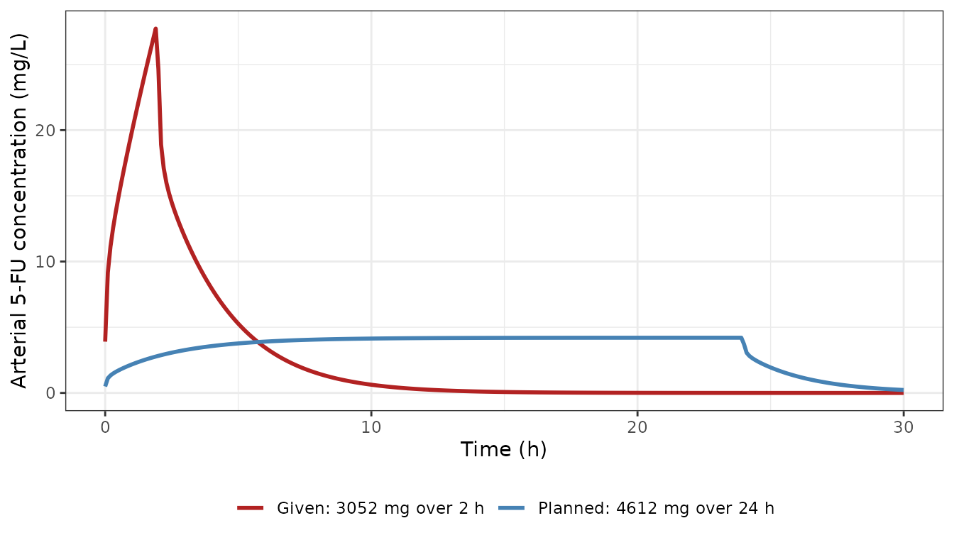
Replicates Figure 2 of Mielke 2025 (central curves; the published bands are not reproduced).
The model gives Cmax 27.7 mg/L and AUC 82.5 mgh/L for the given regimen, and Cmax 4.2 mg/L and AUC 99.5 mgh/L for the planned one. These are the values in Section 2.2.1. The Figure 2 legend’s “AUC as planned 93.1” is the 0-24 h AUC (93.0 here), and the 99.5 of the text is the AUC to 30 h. The checks below compare against those printed values. The model is deterministic, so the only differences are rounding of the published values (to 0.1) and the solver.
given <- patient_summary[grepl("^Given", patient_summary$treatment), ]
planned <- patient_summary[grepl("^Planned", patient_summary$treatment), ]
stopifnot(
  abs(given$cmax - 27.7) < 0.1,
  abs(given$auc_0_30 - 82.5) < 0.1,
  abs(planned$cmax - 4.2) < 0.1,
  abs(planned$auc_0_30 - 99.5) < 0.1,
  abs(planned$auc_0_24 - 93.1) < 0.1
)
Concentration one hour into the infusion
The Discussion recommends sampling one hour after the start of the infusion, when about 50% of the steady-state concentration is reached. Cdyn above 1.5 mg/L would then predict Css above 3 mg/L. For the planned 24 h infusion the model reaches this fraction of its end-of-infusion concentration at 1 h:
PKNCA validation
NCA on the simulated arterial concentrations of the two patient regimens, over 0-30 h, compared with the Cmax and AUC that Section 2.2.1 reports.
conc <- patient |>
  dplyr::filter(!is.na(Cc)) |>
  dplyr::select(id = treatment, time, Cc) |>
  mutate(treatment = id)
doses <- tibble::tribble(
  ~id, ~treatment, ~time, ~amt,
  "Given: 3052 mg over 2 h", "Given: 3052 mg over 2 h", 0, 3052,
  "Planned: 4612 mg over 24 h", "Planned: 4612 mg over 24 h", 0, 4612
)
conc_obj <- PKNCA::PKNCAconc(conc, Cc ~ time | treatment + id)
dose_obj <- PKNCA::PKNCAdose(doses, amt ~ time | treatment + id)
intervals <- data.frame(start = 0, end = 30, cmax = TRUE, tmax = TRUE, auclast = TRUE)
nca_res <- PKNCA::pk.nca(PKNCA::PKNCAdata(conc_obj, dose_obj, intervals = intervals))

published <- tibble::tribble(
  ~treatment, ~cmax, ~auclast,
  "Given: 3052 mg over 2 h", 27.7, 82.5,
  "Planned: 4612 mg over 24 h", 4.2, 99.5
)
cmp <- nlmixr2lib::ncaComparisonTable(
  simulated = nca_res,
  reference = published,
  by = "treatment",
  params = c("cmax", "auclast"),
  units = c(cmax = "mg/L", auclast = "mg*h/L"),
  tolerance_pct = 20
)
knitr::kable(cmp, caption = "Simulated (PKNCA) vs. published (Mielke 2025 Section 2.2.1). * differs from the reference by >20%.")| NCA parameter | treatment | Reference | Simulated | % diff |
|---|---|---|---|---|
| Cmax (mg/L) | Given: 3052 mg over 2 h | 27.7 | 27.7 | +0.1% |
| Cmax (mg/L) | Planned: 4612 mg over 24 h | 4.2 | 4.2 | +0.1% |
| AUClast (mg*h/L) | Given: 3052 mg over 2 h | 82.5 | 82.3 | -0.2% |
| AUClast (mg*h/L) | Planned: 4612 mg over 24 h | 99.5 | 99.5 | -0.0% |
No row differs by more than 20%. PKNCA’s AUC uses the trapezoidal
rule on the 0.1 h grid, so it differs slightly from the integrated
auc_arterial state above.
Model evaluation (Figure 1)
1.0 g IV bolus (Figure 1b, Finch 1979)
A bolus needs a short infusion. Figure 1b starts at about 130 mg/L and peaks near 210 mg/L, and a 0.02 h (72 s) infusion reproduces that. The duration was chosen by the maintainers by reading the panel; the paper does not state it.
bolus_grid <- sort(unique(c(seq(0, 0.02, by = 0.002), seq(0.02, 2, by = 0.01))))
bolus <- solve_infusion(1000, 0.02, bolus_grid, "1.0 g over 0.02 h")
ggplot(bolus, aes(time, Cc)) +
  geom_line(colour = "skyblue3", linewidth = 1) +
  labs(x = "Time (h)", y = "Arterial 5-FU concentration (mg/L)") +
  theme_bw()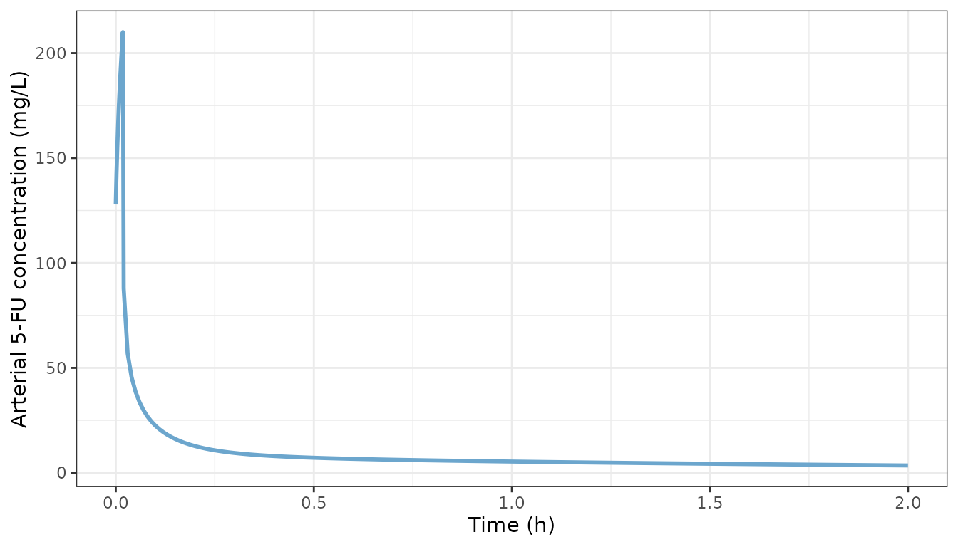
Replicates Figure 1b of Mielke 2025 (model curve only; the Finch 1979 data are not reproduced).
bolus |>
  dplyr::filter(time %in% c(0, 0.0833, 0.5, 1, 2) | Cc == max(Cc)) |>
  dplyr::select(time, Cc) |>
  dplyr::rename("Time (h)" = time, "Cc (mg/L)" = Cc) |>
knitr::kable(digits = 3)| Time (h) | Cc (mg/L) |
|---|---|
| 0.000 | 127.877 |
| 0.018 | 210.015 |
| 0.500 | 7.154 |
| 1.000 | 5.348 |
| 2.000 | 3.484 |
Continuous infusion (Figure 1a, Arshad 2020)
Arshad 2020 gave 650 or 1000 mg/m^2/day as a 5-day continuous infusion. The paper does not say which body-surface area it used to convert these doses for the simulation. Here the Arshad cohort median of 1.95 m^2 is used.
inf_grid <- seq(0, 120, by = 0.5)
bsa <- 1.95
arshad <- bind_rows(
  solve_infusion(650 * bsa * 5, 120, inf_grid, "650 mg/m^2/day"),
  solve_infusion(1000 * bsa * 5, 120, inf_grid, "1000 mg/m^2/day")
)
ggplot(arshad, aes(time, Cc, colour = treatment)) +
  geom_line(linewidth = 1) +
  scale_y_log10() +
  labs(x = "Time (h)", y = "Arterial 5-FU concentration (mg/L)", colour = NULL) +
  theme_bw() +
  theme(legend.position = "bottom")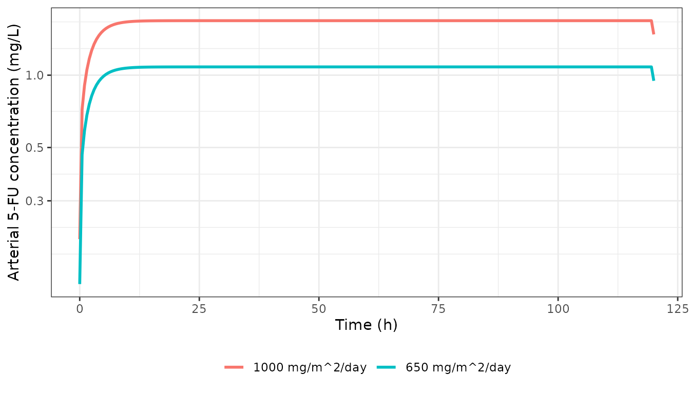
Model at the two Arshad 2020 dose levels (BSA 1.95 m^2), 5-day infusion; compare Figure 1a of Mielke 2025.
arshad |>
  dplyr::filter(time == 100) |>
  dplyr::select(treatment, Cc) |>
  dplyr::rename("Dose level" = treatment, "Cc at 100 h (mg/L)" = Cc) |>
knitr::kable(digits = 3)| Dose level | Cc at 100 h (mg/L) |
|---|---|
| 650 mg/m^2/day | 1.083 |
| 1000 mg/m^2/day | 1.686 |
The model’s plateaus are about 1.1 and 1.7 mg/L. Figure 1a shows plateaus of about 0.19 and 0.29 mg/L, read from the panel by the maintainers. Those are the model’s steady states for 650 and 1000 mg spread over 72 h (about 9.0 and 13.9 mg/h):
per_72h <- bind_rows(
  solve_infusion(650 * 5 / 3, 120, inf_grid, "650 mg per 72 h"),
  solve_infusion(1000 * 5 / 3, 120, inf_grid, "1000 mg per 72 h")
)
per_72h |>
  dplyr::filter(time == 100) |>
  dplyr::select(treatment, Cc) |>
  dplyr::rename("Rate" = treatment, "Cc at 100 h (mg/L)" = Cc) |>
knitr::kable(digits = 3)| Rate | Cc at 100 h (mg/L) |
|---|---|
| 650 mg per 72 h | 0.182 |
| 1000 mg per 72 h | 0.280 |
The panel therefore did not use body-surface-area-scaled doses, and the paper does not state the dose-to-rate conversion behind it. At low concentrations the model’s clearance is about 50 L/h: hepatic blood flow 99.5 L/h in series with an intrinsic clearance of Vmax/Km x Kp = 96 L/h. This is well below the 224-276 L/h that Arshad 2020 estimated and that the paper uses for its variability bands. The model was built and validated for the high concentrations that follow short infusions and overdoses, where clearance is saturated. It over-predicts concentrations from standard-dose continuous infusions.
Assumptions and deviations
-
Script values over Table 1. The deposited script
reproduces every published patient number to the printed precision (Cmax
27.7 and 4.2 mg/L, AUC 82.5 and 99.5 mgh/L, AUC0-24 93.1
mgh/L), so its values are encoded. Table 1 prints a different value
for:
- skeleton volume (6.9 vs 9.33 L);
- red marrow volume (1.2 vs 1.17 L);
- cardiac output (401.7 vs 390 L/h, the sum of the script’s tissue flows);
- the vessel-rich and red-marrow Kp (0.98 and 0.92 vs 0.92 and 0.9).
- Discussion Cmax. The Discussion quotes 4.6 mg/L for the planned schedule. Section 2.2.1, Figure 2 and the script give 4.2 mg/L.
-
Infusion input. The script writes the arterial
input as
Qinf * iv.dose, withiv.doseholding the infusion rate in mg/h andQinf = 1 L/h. The model writes the input directly as the rate (mg/h), which is numerically identical at the published 1 L/h. Because onlyQCof theQC + Qinfarterial outflow reaches the tissues, the structure loses aboutQinf x C_A(about 1 L/h x C_A) of drug. This is part of the published model and is kept. - Blood. There is no blood compartment. The arterial concentration responds instantly to the infusion, so a true bolus is not defined. Figure 1b was reproduced with a 0.02 h infusion chosen from the panel.
- Variability bands. Figures 1 and 2 show bands said to reflect the 224-276 L/h clearance interval of Arshad 2020. The paper does not say how that interval was mapped onto the Michaelis-Menten liver, so the bands are not reproduced and the model carries no IIV.
- Figure 1a. The published curves cannot be reproduced from body-surface-area-scaled doses (see above). The caption also assigns light blue to 650 mg/m^2 although the light-blue curve is the higher one.
- Toxicity analyses. Figures 3-5 (138 Ma et al. dosing records, the literature AUC-derived Css and the decision tree) depend on individual patient data and are not reproduced. The 3 and 6 mg/L thresholds are conclusions of the paper, not model parameters.
- Body weight. The reference adult is 73 kg. The patient was 49 kg, but the script does not scale physiology, so neither does the model.
- No erratum or correction notice was found on EuropePMC as of 2026-11-04.