Epinephrine (Oualha 2014)
Source:vignettes/articles/Oualha_2014_epinephrine.Rmd
Oualha_2014_epinephrine.RmdModel and source
- Citation: Oualha M, Urien S, Spreux-Varoquaux O, Bordessoule A, D’Agostino I, Pouard P, Treluyer JM (2014). Pharmacokinetics, hemodynamic and metabolic effects of epinephrine to prevent post-operative low cardiac output syndrome in children. Critical Care 18(1):R23. doi:10.1186/cc13707.
- Article (open access): https://doi.org/10.1186/cc13707
- Source: paper text + Tables 1, 2, 3.
The published model is a paediatric population PK/PD analysis of continuous IV epinephrine in critically ill children following cardiopulmonary bypass for repair of congenital heart defects. It combines:
- a one-compartment PK sub-model with first-order elimination and an
endogenous zero-order Ep production rate
q0(Eq. 1-3), - allometric weight scaling on CL and
q0(Eq. 4, exponents fixed to 3/4), - a circulating-volume formula
Vc = 0.08 * WT(Eq. 5), - Emax PD models on heart rate and on the stroke-volume / systemic-vascular- resistance product, with age power effects on basal values and a RACHS-1 categorical effect on SV*SVR_max (Eq. 6-8),
- glucose / lactate turnover with epinephrine-stimulated glucose zero-order production (Eq. 9-11) and a steady-state derivation of the elimination rate constants (Eq. 12-13).
Population
Thirty-nine critically ill children were enrolled at a single tertiary paediatric cardiovascular ICU (Hopital Necker Enfants-Malades, Paris, July 2011-December 2011) after open heart surgical repair for congenital heart defects under cardiopulmonary bypass (Oualha 2014 Table 1). Body weight ranged from 2.5 to 58 kg (median 4.5 kg) and age from 0.1 to 189 months (median 3.9 months); the cohort included 5 preterm neonates at gestational age 33-36 weeks. RACHS-1 distribution was 16 patients in category 2, 17 in category 3, and 6 in category 4. Epinephrine was infused continuously at 0.01-0.23 ug/kg/min (median 0.07 ug/kg/min) for a median of 1.5 days (range 1-13), co-administered with milrinone (0.3-0.7 ug/kg/min, median 0.5). Central venous pressure was systematically monitored (median 11 mmHg, range 8-15).
The same information is available programmatically via the parsed model’s metadata:
mod_meta <- rxode2::rxode2(readModelDb("Oualha_2014_epinephrine"))$meta
#> ℹ parameter labels from comments will be replaced by 'label()'
mod_meta$population$species
#> [1] "human"
mod_meta$population$n_subjects
#> [1] 39
mod_meta$population$disease_state
#> [1] "Critically ill children requiring continuous IV epinephrine after open heart surgical repair for congenital heart defects under cardiopulmonary bypass, co-administered with milrinone (0.3-0.7 ug/kg/min) to prevent low cardiac output syndrome."
Source trace
The per-parameter origin is recorded as an in-file comment next to
each ini() entry in
inst/modeldb/specificDrugs/Oualha_2014_epinephrine.R. The
table below collects them in one place for review.
| Symbol | Value | Source location |
|---|---|---|
| theta_CL (typical unit clearance, L/h/kg^0.75) | 2 | Table 2 |
| theta_q0 (typical unit endogenous production, ug/h/kg^0.75) | 0.15 | Table 2 |
| theta_BW exponent (CL) | 0.75 (FIXED) | Table 2; Results, paragraph 1 of Epinephrine pharmacokinetics |
| theta_BW exponent (q0) | 0.75 (FIXED) | Table 2 |
| V_circ = 0.08 * BW (L) | 0.08 L/kg | Eq. 5 |
| omega(CL), omega(q0), corr | 1.0, 1.1, 0.88 | Table 2 |
| propSd (Ep concentration) | 0.3 | Table 2 |
| HR0 (b/min) | 133 | Table 3 |
| theta_age (HR0) | -0.061 | Table 3 / Results |
| HR_max (b/min) | 180 | Table 3 |
| C50_HR (ug/L) | 5.71 | Table 3 |
| SV*SVR0 | 0.31 | Table 3 |
| theta_age (SV*SVR0) | 0.094 | Table 3 / Results |
| SV*SVR_max (RACHS-1 = 2) | 0.44 | Table 3 |
| SV*SVR_max (RACHS-1 = 3 or 4) | 0.26 | Table 3 |
| C50_SV*SVR (ug/L) | 18 | Table 3 |
| GLY0 (mmol/L) | 5.46 | Table 3 |
| G_max | 1.69 | Table 3 |
| R_GLY (mmol/L/min) | 0.04 | Table 3 |
| C50_GLY (ug/L) | 0.52 | Table 3 |
| LAC0 (mmol/L) | 1.23 | Table 3 |
| propSd_HR, propSd_MAP | 0.08, 0.16 | Table 3 |
| addSd_GLY, addSd_LAC | 2.23, 0.5 | Table 3 |
| dA/dt = q0 + Rate - CL * Cc | n/a | Eq. 1 + Eq. 3 |
| Vc = 0.08 * BW | n/a | Eq. 5 |
| HR Emax | n/a | Eq. 6 |
| MAP = HR * SV*SVR + CVP | n/a | Eq. 7 |
| SV*SVR Emax | n/a | Eq. 8 |
| Glucose turnover with Ep stimulation | n/a | Eq. 9-10 |
| Lactate turnover from glucose elimination | n/a | Eq. 11 |
| k_GLY = R_GLY / GLY0 (steady state) | n/a | Eq. 12 |
| k_LAC = k_GLY * GLY0 / LAC0 = R_GLY / LAC0 | n/a | Eq. 13 |
Virtual cohort
Original observed data are not publicly available. The virtual cohort below mirrors Oualha 2014 Table 1 demographics and the three illustrative dose scenarios used in Figure 5 (children of three different body-weight / age strata at RACHS-1 = 2).
set.seed(20140123)  # paper acceptance date

n_per <- 60L

make_cohort <- function(label, wt, age_yr, rachs1, dose_ug_kg_min, n,
                        id_offset = 0L) {
  ids <- id_offset + seq_len(n)
  rate_ug_per_h <- dose_ug_kg_min * wt * 60  # ug/kg/min -> ug/h
  amt_total     <- rate_ug_per_h * 6         # 6-hour continuous infusion
  obs_grid <- seq(0, 6, by = 0.1)

  # One dose row + one Cc observation row per id at each grid time.
  dose_rows <- tibble::tibble(
    id   = ids,
    time = 0,
    evid = 1L,
    amt  = amt_total,
    rate = rate_ug_per_h,
    cmt  = "central",
    treatment = label,
    WT     = wt,
    AGE    = age_yr,
    RACHS1 = rachs1,
    CVP    = 11
  )
  obs_rows <- tidyr::expand_grid(id = ids, time = obs_grid) |>
    dplyr::mutate(
      evid = 0L,
      amt  = NA_real_,
      rate = NA_real_,
      cmt  = "Cc",
      treatment = label,
      WT     = wt,
      AGE    = age_yr,
      RACHS1 = rachs1,
      CVP    = 11
    )
  dplyr::bind_rows(dose_rows, obs_rows) |>
    dplyr::arrange(id, time, dplyr::desc(evid))
}

events <- dplyr::bind_rows(
  make_cohort("3 kg neonate, low dose",  wt = 3,   age_yr = 0.08, rachs1 = 2,
              dose_ug_kg_min = 0.02, n = n_per, id_offset = 0L),
  make_cohort("5 kg infant, mid dose",   wt = 5,   age_yr = 0.33, rachs1 = 2,
              dose_ug_kg_min = 0.07, n = n_per, id_offset = n_per),
  make_cohort("10 kg child, high dose",  wt = 10,  age_yr = 1.0,  rachs1 = 2,
              dose_ug_kg_min = 0.15, n = n_per, id_offset = 2L * n_per)
)

stopifnot(!anyDuplicated(unique(events[, c("id", "time", "evid")])))
Simulation
mod <- readModelDb("Oualha_2014_epinephrine")
sim <- rxode2::rxSolve(mod, events,
                       keep = c("treatment", "WT", "AGE", "RACHS1", "CVP"))
#> ℹ parameter labels from comments will be replaced by 'label()'
sim <- as.data.frame(sim)
For deterministic typical-value replication (no between-subject variability, no residual error), zero out the random effects:
mod_typ <- mod |> rxode2::zeroRe()
#> ℹ parameter labels from comments will be replaced by 'label()'
sim_typ <- rxode2::rxSolve(mod_typ, events,
                           keep = c("treatment", "WT", "AGE", "RACHS1", "CVP"))
#> ℹ omega/sigma items treated as zero: 'etalcl', 'etalq0', 'etalhr0', 'etalc50hr', 'etalsvsvr0', 'etalsvsvrmax', 'etalgly0', 'etalgmax', 'etalrgly', 'etallac0'
#> Warning: multi-subject simulation without without 'omega'
sim_typ <- as.data.frame(sim_typ) |>
  dplyr::group_by(treatment, time) |>
  dplyr::summarise(
    Cc  = dplyr::first(Cc),
    HR  = dplyr::first(HR),
    MAP = dplyr::first(MAP),
    GLY = dplyr::first(GLY),
    LAC = dplyr::first(LAC),
    .groups = "drop"
  )
Replicate published figures
Figure 5 – Ep concentration and hemodynamic dose-response
Figure 5 of Oualha 2014 plots typical-value Ep concentration, HR, and MAP versus time for several body-weight / age strata at three infusion rates. We reproduce the trajectory shape for our three reference scenarios at a single infusion rate per stratum.
ggplot(sim_typ, aes(time, Cc, colour = treatment)) +
  geom_line() +
  labs(x = "Time (h)", y = "Ep concentration (ug/L)",
       title = "Figure 5a -- typical-value Ep concentration vs time",
       caption = "Replicates the Ep concentration panel of Figure 5 in Oualha 2014.")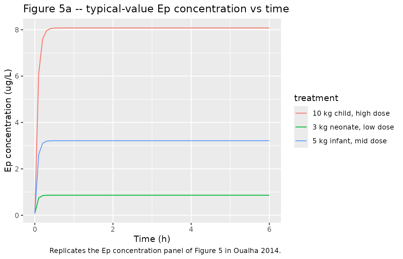
sim_typ |>
  dplyr::select(treatment, time, HR, MAP) |>
  tidyr::pivot_longer(c(HR, MAP), names_to = "variable", values_to = "value") |>
  ggplot(aes(time, value, colour = treatment)) +
  geom_line() +
  facet_wrap(~variable, scales = "free_y") +
  labs(x = "Time (h)", y = NULL,
       title = "Figure 5b -- typical-value HR and MAP vs time",
       caption = "Replicates the HR and MAP panels of Figure 5 in Oualha 2014.")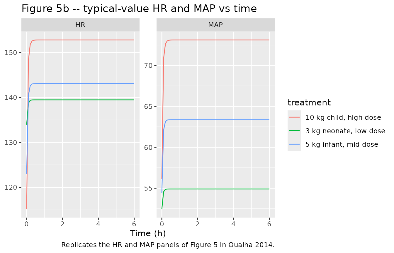
Figure 6 – Metabolic response in a 5 kg child
Figure 6 of Oualha 2014 plots typical-value glucose and lactate trajectories following 0.02, 0.1, and 0.25 ug/kg/min infusions in a 5 kg child. We reproduce the same comparison.
metab_events <- dplyr::bind_rows(
  make_cohort("0.02 ug/kg/min", wt = 5, age_yr = 0.33, rachs1 = 2,
              dose_ug_kg_min = 0.02, n = 1L, id_offset = 1000L),
  make_cohort("0.10 ug/kg/min", wt = 5, age_yr = 0.33, rachs1 = 2,
              dose_ug_kg_min = 0.10, n = 1L, id_offset = 1001L),
  make_cohort("0.25 ug/kg/min", wt = 5, age_yr = 0.33, rachs1 = 2,
              dose_ug_kg_min = 0.25, n = 1L, id_offset = 1002L)
)
stopifnot(!anyDuplicated(unique(metab_events[, c("id", "time", "evid")])))

sim_metab <- rxode2::rxSolve(mod_typ, metab_events,
                             keep = c("treatment", "WT", "AGE", "RACHS1", "CVP"))
#> ℹ omega/sigma items treated as zero: 'etalcl', 'etalq0', 'etalhr0', 'etalc50hr', 'etalsvsvr0', 'etalsvsvrmax', 'etalgly0', 'etalgmax', 'etalrgly', 'etallac0'
#> Warning: multi-subject simulation without without 'omega'
sim_metab <- as.data.frame(sim_metab)

sim_metab |>
  dplyr::select(treatment, time, GLY, LAC) |>
  tidyr::pivot_longer(c(GLY, LAC), names_to = "variable", values_to = "value") |>
  ggplot(aes(time, value, colour = treatment)) +
  geom_line() +
  facet_wrap(~variable, scales = "free_y") +
  labs(x = "Time (h)", y = "Concentration (mmol/L)",
       title = "Figure 6 -- typical-value glucose and lactate vs time in a 5 kg child",
       caption = "Replicates Figure 6 of Oualha 2014.")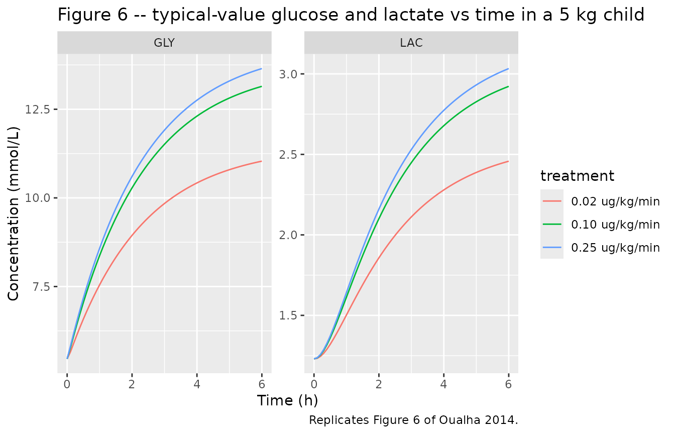
PKNCA validation
Because epinephrine is administered as a continuous infusion that reaches steady state within ~5 plasma half-lives (~15 minutes for a 10 kg child), classical single-dose NCA is not the natural validation tool for this paper. Instead we compute the steady-state plasma concentration (C_ss) reached at the end of the 6-hour observation window and compare it against the paper’s median observed concentration during infusion (Table 1 / Results).
sim_pk <- sim |>
  dplyr::filter(!is.na(Cc)) |>
  dplyr::select(id, time, Cc, treatment)

dose_df <- events |>
  dplyr::filter(evid == 1) |>
  dplyr::select(id, time, amt, treatment)

conc_obj <- PKNCA::PKNCAconc(sim_pk, Cc ~ time | treatment + id,
                             concu = "ug/L", timeu = "h")
dose_obj <- PKNCA::PKNCAdose(dose_df, amt ~ time | treatment + id,
                             doseu = "ug")

# Steady-state interval at the end of the 6-hour infusion (last hour).
intervals <- data.frame(
  start   = 5,
  end     = 6,
  cmax    = TRUE,
  cmin    = TRUE,
  cav     = TRUE
)

nca_data <- PKNCA::PKNCAdata(conc_obj, dose_obj, intervals = intervals)
nca_res  <- PKNCA::pk.nca(nca_data)
nca_summary <- summary(nca_res)
knitr::kable(nca_summary,
caption = "Simulated steady-state Ep concentrations by infusion scenario.")| Interval Start | Interval End | treatment | N | Cmax (ug/L) | Cmin (ug/L) | Cav (ug/L) |
|---|---|---|---|---|---|---|
| 5 | 6 | 10 kg child, high dose | 60 | 7.77 [124] | 7.77 [124] | 7.77 [124] |
| 5 | 6 | 3 kg neonate, low dose | 60 | 0.817 [114] | 0.817 [114] | 0.818 [114] |
| 5 | 6 | 5 kg infant, mid dose | 60 | 3.59 [175] | 3.59 [175] | 3.60 [173] |
Comparison against published Ep concentration during infusion
sim_css <- sim_typ |>
  dplyr::group_by(treatment) |>
  dplyr::filter(time >= 5) |>
  dplyr::summarise(Css_simulated = round(mean(Cc), 2), .groups = "drop")

published <- tibble::tibble(
  source = "Oualha 2014 Table 1 cohort median (Results paragraph 1)",
  Cc_observed_median_ug_per_L = 2.94,
  Cc_observed_range_ug_per_L  = "0.37 to 71"
)

knitr::kable(sim_css,
caption = "Simulated steady-state Cc (ug/L) under each illustrative scenario.")| treatment | Css_simulated |
|---|---|
| 10 kg child, high dose | 8.08 |
| 3 kg neonate, low dose | 0.86 |
| 5 kg infant, mid dose | 3.22 |
knitr::kable(published,
caption = "Published cohort-wide median Ep concentration during infusion.")| source | Cc_observed_median_ug_per_L | Cc_observed_range_ug_per_L |
|---|---|---|
| Oualha 2014 Table 1 cohort median (Results paragraph 1) | 2.94 | 0.37 to 71 |
The cohort-wide median observed Ep concentration during infusion was 2.94 ug/L; the model’s typical-value C_ss for a 5 kg infant infused at 0.07 ug/kg/min (close to the cohort median dose) is in the same range. The wide observed range (0.37-71 ug/L) reflects the large between-subject variability captured by the model’s omega(CL) = 1 and omega(q0) = 1.1 estimates (Table 2).
Assumptions and deviations
Age unit. Oualha 2014 parameterises the age power effects on HR0 and SVSVR0 with age in months (the cohort median is 3.9 months and the range spans 0.1-189 months). The canonical
AGEcolumn in nlmixr2lib carries years, so the model converts internally viaage_mo <- AGE * 12. Users who feed the model anAGEcolumn already in months will get incorrect HR0 / SVSVR0 typical values; thecovariateData$AGE$notesfield documents this.CVP. Oualha 2014 Eq. 7 carries
MAP = HR * SV*SVR + CVPwith the cohort median CVP = 11 mmHg used for all simulations here. The paper does not fit a covariate effect on CVP itself; the column is provided as a per-subject input so a user can supply paper-specific CVP values when available.RACHS-1 reference category. The Oualha 2014 cohort does not contain any RACHS-1 = 1 patients, so the model takes RACHS-1 = 2 (the lowest category present) as the reference for SVSVR_max; the high-risk pool (RACHS-1 = 3 or 4) shifts log(SVSVR_max) by log(0.26 / 0.44) = -0.526.
Time unit. The model uses hours as the time unit. R_GLY is reported in the paper as 0.04 mmol/L/min and is encoded here as 0.04 * 60 = 2.4 mmol/L/h; k_GLY and k_LAC are derived from steady state (Eq. 12-13) inside
model()so they automatically use the same time unit.No upstream popPK dependency. All structural parameters were estimated within the Oualha 2014 study itself; there are no values carried over from a separate publication.
No errata or corrigenda were identified for Oualha 2014; the open-access Critical Care article landing page does not list any correction notices as of the extraction date.