Attarwala_2023_mRNA3927 • nlmixr2lib

Model and source

Citation: Attarwala H, Lumley M, Liang M, Ivaturi V, Senn J. Translational Pharmacokinetic/Pharmacodynamic Model for mRNA-3927, an Investigational Therapeutic for the Treatment of Propionic Acidemia. Nucleic Acid Ther. 2023;33(2):141-147. doi:10.1089/nat.2022.0036
Description: Preclinical (mouse, rat, cynomolgus monkey; allometrically scalable to humans). Translational semi-mechanistic PK and PK/PD model for mRNA-3927, an LNP-encapsulated dual mRNA encoding propionyl-CoA carboxylase (PCC) subunits PCCA and PCCB. PK: 3-compartment plasma1-tissue-plasma2 redistribution (V shared between the two plasma compartments; V and V2 fixed at the mouse reference and scaled allometrically) with body-weight allometric scaling of clearances (mouse reference 0.025 kg; estimated exponents cla on CL12/CL32 and clb on CL23/CL20). PD: liver PCC protein 2-compartment indirect-response model driven by an effect compartment linked to plasma mRNA, with synthesis linear in effect-compartment mRNA concentration and first-order degradation. Three downstream biomarkers (2-methylcitrate, 3-hydroxypropionate, C3/C2 carnitine ratio) follow direct sigmoidal Imax suppression by liver PCC protein with Imax fixed at 0.999.
Article: https://doi.org/10.1089/nat.2022.0036
PMC supplements:
- Supplementary Table S1 (model equations): https://www.ebi.ac.uk/europepmc/webservices/rest/PMC10066765/supplementaryFiles
- Supplementary Figures S1-S3 (individual fits): same archive

mRNA-3927 is an investigational lipid-nanoparticle (LNP) drug product containing two messenger RNAs that encode the PCCA and PCCB subunits of propionyl-CoA carboxylase (PCC), the deficient enzyme in propionic acidemia (PA). The translational PK/PD model in Attarwala 2023 was fit jointly across mouse, rat, and cynomolgus monkey PK data, then extrapolated allometrically to humans to support first-in-human dose selection for the Phase 1/2 study NCT04159103.

Population

The published model is anchored to preclinical data (Attarwala 2023, Methods, p. 142):

PCC-deficient mice (strain 4011020 (A138T) PCCA -/-), N = 111. Body weight reference: 0.025 kg.
Juvenile Sprague-Dawley rats, N = 19. Body weight: not tabulated; typical juvenile SD rat ~0.20 kg.
Cynomolgus monkeys, N = 16. Body weight: not tabulated; typical cyno ~3 kg.

PCC pharmacodynamic data (PCC protein time-course; 2-MC, 3-HP, C3/C2 ratio biomarkers) are mouse-only. The interspecies PK fit drives the human-extrapolation use case described in the Discussion (Attarwala 2023, p. 145).

Source trace

Parameter origin is recorded in-file alongside each ini() entry. The table below lists each parameter and its source location.

Per-parameter source trace for the PK and PD layers.
Parameter	Value (mouse reference)	Source
lcl12 = log(19.7)	CL12 = 19.7 mL/h	Attarwala 2023 Table 1, RSE 23.1%
lcl23 = log(0.215)	CL23 = 0.215 mL/h	Attarwala 2023 Table 1, RSE 35.9%
lcl32 = log(2.96)	CL32 = 2.96 mL/h	Attarwala 2023 Table 1, RSE 48.2%
lcl20 = log(0.136)	CL20 = 0.136 mL/h	Attarwala 2023 Table 1, RSE 3.78%
lvc = fixed(log(2.67))	V (plasma1, plasma2) = 2.67 mL	Attarwala 2023 Table 1 footnote f, fixed
lvp = fixed(log(0.961))	V2 (tissue) = 0.961 mL	Attarwala 2023 Table 1 footnote f, fixed
e_wt_cla = 0.631	Allometric exp on CL12 / CL32	Attarwala 2023 Table 1, RSE 9.2%
e_wt_clb = 1.10	Allometric exp on CL23 / CL20	Attarwala 2023 Table 1, RSE 7.55%
etalcl32 ~ 0.245	IIV on CL32 = 52.7% CV	Attarwala 2023 Table 1; log(1 + 0.527^2) = 0.245
propSd = 0.375	Proportional residual on plasma mRNA = 37.5%	Attarwala 2023 Table 1, RSE 11.0%
lke0 = log(0.242)	ke0 = 0.242 /h	Attarwala 2023 Table 1, RSE 3.35%
lslope = log(55.6)	Slope = 55.6 (mg/g/h)/(mg/mL)	Attarwala 2023 Table 1, RSE 1.93%
lkdeg = log(0.0075)	kdeg = 0.0075 /h	Attarwala 2023 Table 1, RSE 2.82%
lkq = log(0.00474)	kq = 0.00474 /h	Attarwala 2023 Table 1, RSE 6.7%
propSd_PCC = 0.305	Proportional residual on PCC = 30.5%	Attarwala 2023 Table 1, RSE 0.02%
imax = fixed(0.999)	Imax = 0.999 (fixed)	Attarwala 2023 Table 1 footnote m
le0_mc2 = log(1.67)	E0 2-MC = 1.67 umol/L	Attarwala 2023 Table 1, RSE 4.46%
lbase_mc2 = log(2.93)	2-MC suppressible baseline = 2.93 umol/L	Attarwala 2023 Table 1, RSE 6.66%
lic50_mc2 = log(21.0)	IC50 2-MC = 21.0 (PCC mass per liver tissue)	Attarwala 2023 Table 1, RSE 8.96%
etale0_mc2 ~ 0.0862	IIV E0 2-MC = 30.0% CV	Attarwala 2023 Table 1; log(1 + 0.300^2) = 0.0862
etalbase_mc2 ~ 0.1874	IIV base 2-MC = 45.4% CV	Attarwala 2023 Table 1; log(1 + 0.454^2) = 0.1874
propSd_MC2 = 0.234	Proportional residual 2-MC = 23.4%	Attarwala 2023 Table 1, RSE 3.84%
le0_hp3 = log(0.0987)	E0 3-HP = 0.0987 umol/L	Attarwala 2023 Table 1, RSE 6.74%
lbase_hp3 = log(60.1)	3-HP suppressible baseline = 60.1 umol/L	Attarwala 2023 Table 1, RSE 14.4%
lic50_hp3 = log(37.5)	IC50 3-HP = 37.5 (PCC mass per liver tissue)	Attarwala 2023 Table 1, RSE 12.2%
etale0_hp3 ~ 0.2320	IIV E0 3-HP = 51.1% CV	Attarwala 2023 Table 1; log(1 + 0.511^2) = 0.2320
etalbase_hp3 ~ 0.4348	IIV base 3-HP = 73.8% CV	Attarwala 2023 Table 1; log(1 + 0.738^2) = 0.4348
propSd_HP3 = 0.348	Proportional residual 3-HP = 34.8%	Attarwala 2023 Table 1, RSE 5.56%
le0_c3c2 = log(0.347)	E0 C3/C2 = 0.347 umol/L	Attarwala 2023 Table 1, RSE 6.4%
lbase_c3c2 = log(2.31)	C3/C2 suppressible baseline = 2.31 umol/L	Attarwala 2023 Table 1, RSE 6.61%
lic50_c3c2 = log(32.1)	IC50 C3/C2 = 32.1 (PCC mass per liver tissue)	Attarwala 2023 Table 1, RSE 11.7%
etale0_c3c2 ~ 0.2385	IIV E0 C3/C2 = 51.9% CV	Attarwala 2023 Table 1; log(1 + 0.519^2) = 0.2385
etalbase_c3c2 ~ 0.2762	IIV base C3/C2 = 56.4% CV	Attarwala 2023 Table 1; log(1 + 0.564^2) = 0.2762
propSd_C3C2 = 0.360	Proportional residual C3/C2 = 36.0%	Attarwala 2023 Table 1, RSE 4.79%

The structural equations come from Supplementary Table S1:

Block	Equation
(A) PK	`d(A1)/dt = input - CL12 * C1`; `d(A2)/dt = CL12 * C1 - CL23 * C2 + CL32 * C3 - CL20 * C2`; `d(A3)/dt = CL23 * C2 - CL32 * C3`; observation `C13 = C1 + C3`
(A) Allometric	`CL12 = tvCL12 * (BW / 0.025)^cla`; same exponent on CL32. `CL23 = tvCL23 * (BW / 0.025)^clb`; same exponent on CL20. `V = tvV * (BW / 0.025)^1`; `V2 = tvV2 * (BW / 0.025)^1`.
(B) PD effect	`d(Ce)/dt = Ke0 * (C13 - Ce)`
(B) PCC protein	`d(PCC)/dt = Slope * Ce + Kq * (PCP - PCC) - Kdeg * PCC`; `d(PCP)/dt = Kq * (PCC - PCP)`
(C) Biomarkers	for each B in {2-MC, 3-HP, C3/C2}: `B = E0_B + base_B * (1 - Imax * PCC / (IC50_B + PCC))`, Imax fixed at 0.999.

Virtual cohort

We replicate Figure 2A by simulating typical-individual time profiles at each species-dose combination reported in Attarwala 2023 (mouse 1 and 2 mg/kg; rat 1, 3, 9 mg/kg; monkey 1, 3, 5 mg/kg). The simulation uses the package’s typical-value parameterisation (no IIV, no residual error) so each cohort profile is a single deterministic trace driven by the published parameter estimates.

make_cohort <- function(id, species, body_weight_kg, dose_mg_per_kg,
                        t_obs, dose_times_h = 0) {
  amt_mg <- dose_mg_per_kg * body_weight_kg
  dose_rows <- tibble::tibble(
    id    = id,
    time  = dose_times_h,
    amt   = amt_mg,
    evid  = 1L,
    cmt   = "central",
    WT    = body_weight_kg,
    species = species,
    dose_label = sprintf("%s %s mg/kg", species, format(dose_mg_per_kg))
  )
  obs_rows <- tibble::tibble(
    id    = id,
    time  = t_obs,
    amt   = 0,
    evid  = 0L,
    cmt   = "Cc",
    WT    = body_weight_kg,
    species = species,
    dose_label = sprintf("%s %s mg/kg", species, format(dose_mg_per_kg))
  )
  dplyr::bind_rows(dose_rows, obs_rows) |>
    dplyr::arrange(time, dplyr::desc(evid))
}

# Single-dose PK cohorts (Attarwala 2023 Figure 2A):
#   mouse  0-48 h    after 1 / 2 mg/kg
#   rat    0-96 h    after 1 / 3 / 9 mg/kg
#   monkey 0-96 h    after 1 / 3 / 5 mg/kg
t_mouse  <- c(0.01, seq(0.5, 48,  length.out = 80))
t_animal <- c(0.01, seq(0.5, 96,  length.out = 80))

cohorts_pk <- dplyr::bind_rows(
  make_cohort(  1L, "mouse",   0.025, 1, t_obs = t_mouse),
  make_cohort(  2L, "mouse",   0.025, 2, t_obs = t_mouse),
  make_cohort(  3L, "rat",     0.20,  1, t_obs = t_animal),
  make_cohort(  4L, "rat",     0.20,  3, t_obs = t_animal),
  make_cohort(  5L, "rat",     0.20,  9, t_obs = t_animal),
  make_cohort(  6L, "monkey",  3.0,   1, t_obs = t_animal),
  make_cohort(  7L, "monkey",  3.0,   3, t_obs = t_animal),
  make_cohort(  8L, "monkey",  3.0,   5, t_obs = t_animal)
)
stopifnot(!anyDuplicated(unique(cohorts_pk[, c("id", "time", "evid")])))

Simulation

mod_typical <- readModelDb("Attarwala_2023_mRNA3927") |> rxode2::zeroRe()
#> ℹ parameter labels from comments will be replaced by 'label()'

sim_pk <- rxode2::rxSolve(
  mod_typical,
  events = cohorts_pk,
  keep   = c("species", "dose_label")
) |> as.data.frame()
#> ℹ omega/sigma items treated as zero: 'etalcl32', 'etale0_mc2', 'etalbase_mc2', 'etale0_hp3', 'etalbase_hp3', 'etale0_c3c2', 'etalbase_c3c2'
#> Warning: multi-subject simulation without without 'omega'

Figure 2A – plasma mRNA across species and doses

Attarwala 2023 Figure 2A shows observed plus fitted plasma mRNA concentrations on a log y-axis for mouse 1 / 2 mg/kg, rat 1 / 3 / 9 mg/kg, and monkey 1 / 3 / 5 mg/kg. The figure below reproduces the typical-value model trajectories for each cohort. Concentration units follow Supplementary Table S1 (V in mL, dose in mg, so Cc in mg/mL). Observed-data overlays are not available because the preclinical dataset has not been released; this figure replicates the “population predicted” black curve in Figure 2A.

sim_pk |>
  dplyr::filter(time > 0) |>
  ggplot(aes(time, Cc, group = dose_label, colour = dose_label)) +
  geom_line() +
  facet_wrap(~ species, scales = "free", nrow = 1) +
  scale_y_log10() +
  labs(x = "Time after dose (h)", y = "Plasma mRNA Cc (mg/mL)",
       colour = "Cohort",
       title = "Figure 2A replication -- plasma PCCA / PCCB mRNA across species",
       caption = "Typical-individual simulation; Attarwala 2023 Fig 2A.")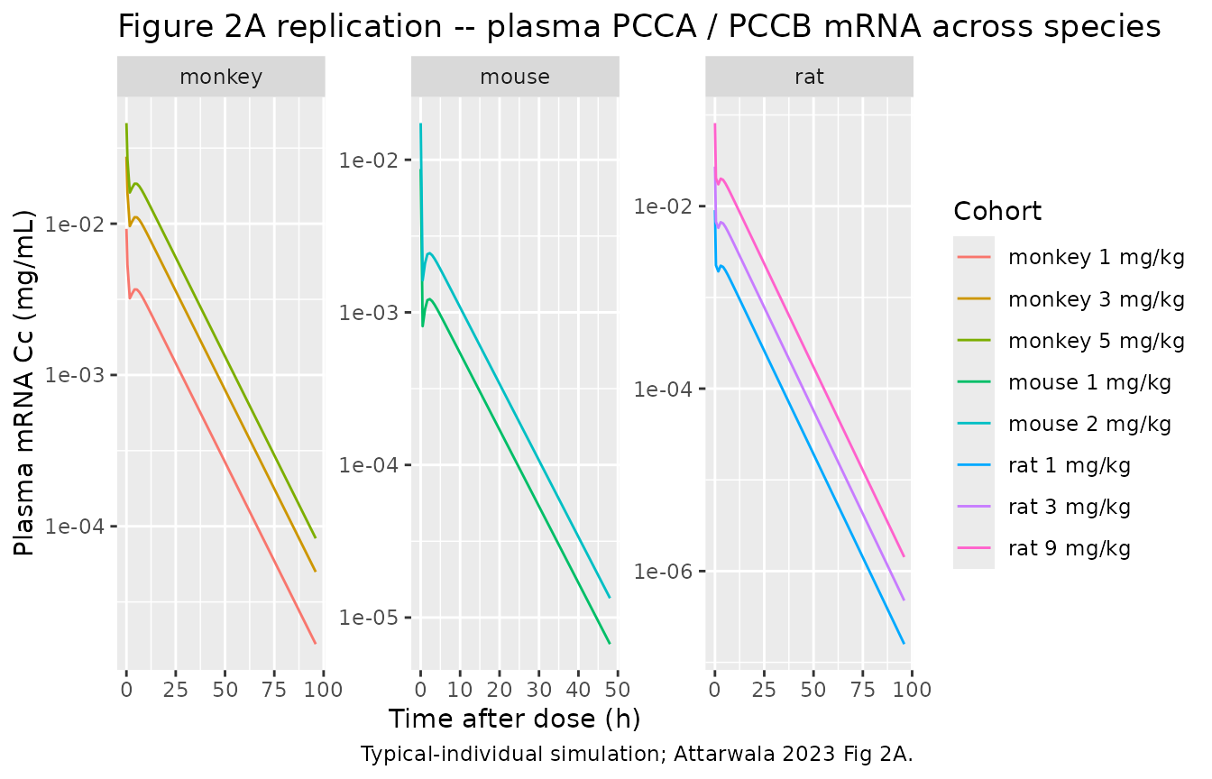

Figure 2B – liver PCC protein time course after a single 1 mg/kg IV bolus in PCC-deficient mice

t_pcc <- seq(0, 21, by = 0.25) * 24  # 0-21 days, expressed in hours

pcc_dose <- tibble::tibble(id = 1L, time = 0, amt = 0.025, evid = 1L,
                            cmt = "central", WT = 0.025)
pcc_obs  <- tibble::tibble(id = 1L, time = t_pcc, amt = 0, evid = 0L,
                            cmt = "PCC", WT = 0.025)
pcc_events <- dplyr::bind_rows(pcc_dose, pcc_obs) |>
  dplyr::arrange(time, dplyr::desc(evid))

sim_pcc <- rxode2::rxSolve(mod_typical, events = pcc_events) |> as.data.frame()
#> ℹ omega/sigma items treated as zero: 'etalcl32', 'etale0_mc2', 'etalbase_mc2', 'etale0_hp3', 'etalbase_hp3', 'etale0_c3c2', 'etalbase_c3c2'

ggplot(sim_pcc |> dplyr::mutate(day = time / 24), aes(day, PCC)) +
  geom_line() +
  scale_y_log10() +
  labs(x = "Time (days)", y = "Liver PCC protein (mass per liver tissue)",
       title = "Figure 2B replication -- liver PCC protein after 1 mg/kg IV mRNA-3927",
       caption = "Typical-individual simulation in PCC-deficient mouse (WT = 0.025 kg).")
#> Warning in scale_y_log10(): log-10 transformation introduced
#> infinite values.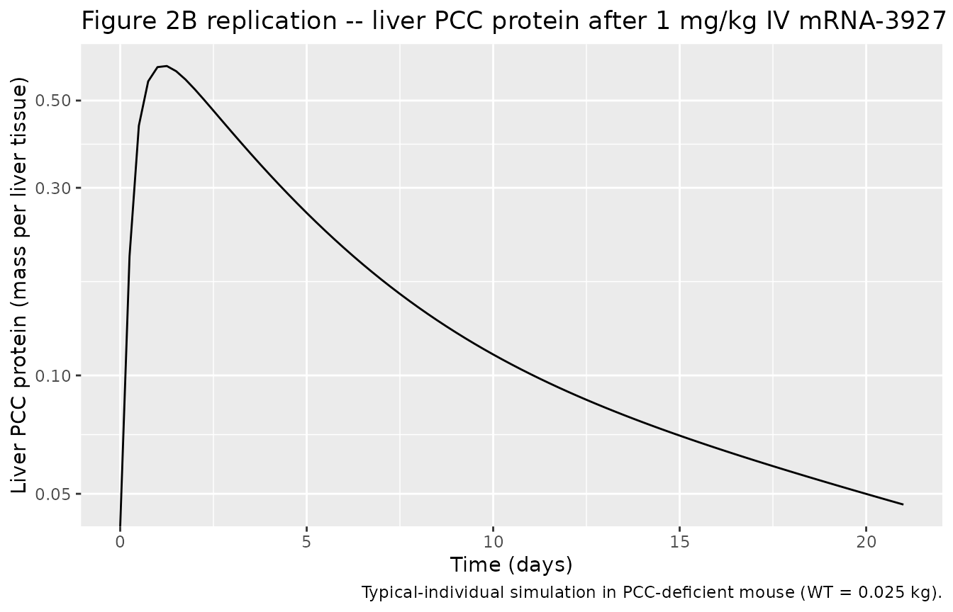

Q3W multi-dose biomarker dynamics in mice

Figure 3 and Supplementary Figures S1-S3 in Attarwala 2023 show 2-MC, 3-HP, and C3/C2 ratio responses after q3W dosing of mRNA-3927 in PCC-deficient mice. Below we simulate the 2 mg/kg q3W x 4 cohort and plot the three plasma biomarkers; the paper reports near-maximal suppression at q3W doses of >= 2 mg/kg.

q3w_times_h <- (0:3) * 21 * 24
biom_obs_h  <- seq(0, 12 * 7, by = 0.5) * 24  # 0-84 days, every 12 h

biom_events <- dplyr::bind_rows(
  tibble::tibble(id = 1L, time = q3w_times_h, amt = 0.025 * 2, evid = 1L,
                  cmt = "central", WT = 0.025),
  tibble::tibble(id = 1L, time = biom_obs_h, amt = 0, evid = 0L,
                  cmt = "MC2", WT = 0.025),
  tibble::tibble(id = 1L, time = biom_obs_h, amt = 0, evid = 0L,
                  cmt = "HP3", WT = 0.025),
  tibble::tibble(id = 1L, time = biom_obs_h, amt = 0, evid = 0L,
                  cmt = "C3C2", WT = 0.025)
) |> dplyr::arrange(time, dplyr::desc(evid))

sim_biom <- rxode2::rxSolve(mod_typical, events = biom_events) |>
  as.data.frame()
#> ℹ omega/sigma items treated as zero: 'etalcl32', 'etale0_mc2', 'etalbase_mc2', 'etale0_hp3', 'etalbase_hp3', 'etale0_c3c2', 'etalbase_c3c2'

biom_long <- sim_biom |>
  dplyr::select(time, MC2, HP3, C3C2) |>
  tidyr::pivot_longer(c(MC2, HP3, C3C2), names_to = "biomarker", values_to = "value") |>
  dplyr::mutate(day = time / 24)

ggplot(biom_long, aes(day, value)) +
  geom_line() +
  facet_wrap(~ biomarker, scales = "free_y") +
  labs(x = "Time (days)", y = "Biomarker (umol/L)",
       title = "Q3W 2 mg/kg mRNA-3927 in PCC-deficient mice -- plasma biomarkers",
       caption = "Typical-individual simulation; replicates Attarwala 2023 Suppl. Figs S1-S3.")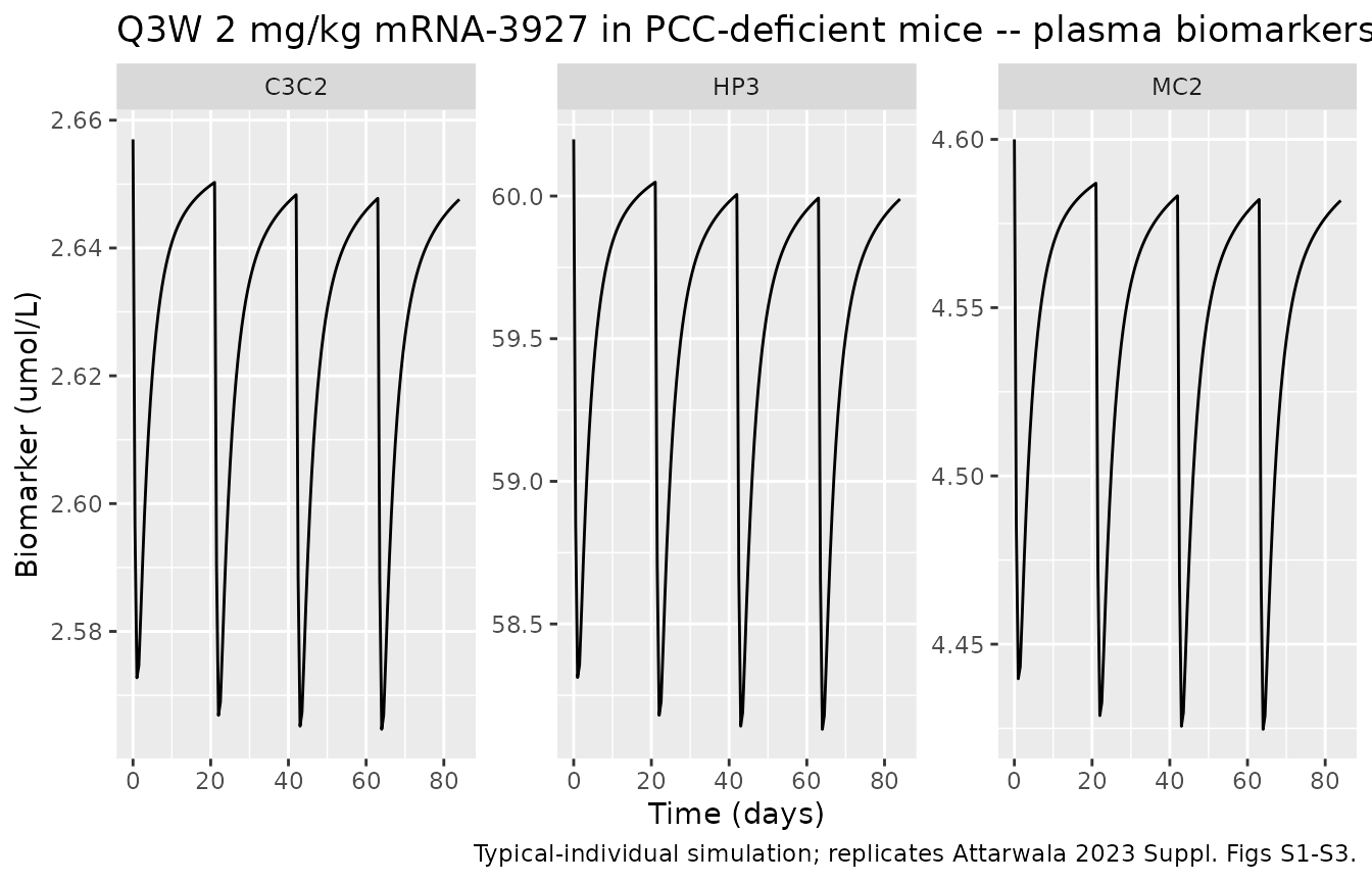

Human allometric extrapolation

The paper’s stated use of the model is to extrapolate to humans by setting body weight in the allometric scaling expressions to a human value (Discussion, p. 145). We illustrate a 70 kg adult receiving 1 mg/kg IV mRNA-3927 over 21 days; both plasma mRNA (Cc) and liver PCC protein (PCC) are shown.

t_human_h <- seq(0, 21, by = 0.25) * 24
human_events <- dplyr::bind_rows(
  tibble::tibble(id = 1L, time = 0,        amt = 70, evid = 1L,
                  cmt = "central", WT = 70),
  tibble::tibble(id = 1L, time = t_human_h, amt = 0, evid = 0L,
                  cmt = "Cc",  WT = 70),
  tibble::tibble(id = 1L, time = t_human_h, amt = 0, evid = 0L,
                  cmt = "PCC", WT = 70)
) |> dplyr::arrange(time, dplyr::desc(evid))

sim_human <- rxode2::rxSolve(mod_typical, events = human_events) |>
  as.data.frame()
#> ℹ omega/sigma items treated as zero: 'etalcl32', 'etale0_mc2', 'etalbase_mc2', 'etale0_hp3', 'etalbase_hp3', 'etale0_c3c2', 'etalbase_c3c2'

sim_human |>
  dplyr::filter(time > 0) |>
  dplyr::mutate(day = time / 24) |>
  tidyr::pivot_longer(c(Cc, PCC), names_to = "Output", values_to = "Value") |>
  ggplot(aes(day, Value)) +
  geom_line() +
  facet_wrap(~ Output, scales = "free_y") +
  scale_y_log10() +
  labs(x = "Time (days)", y = "Output value",
       title = "Allometric extrapolation -- 70 kg adult, 1 mg/kg IV mRNA-3927")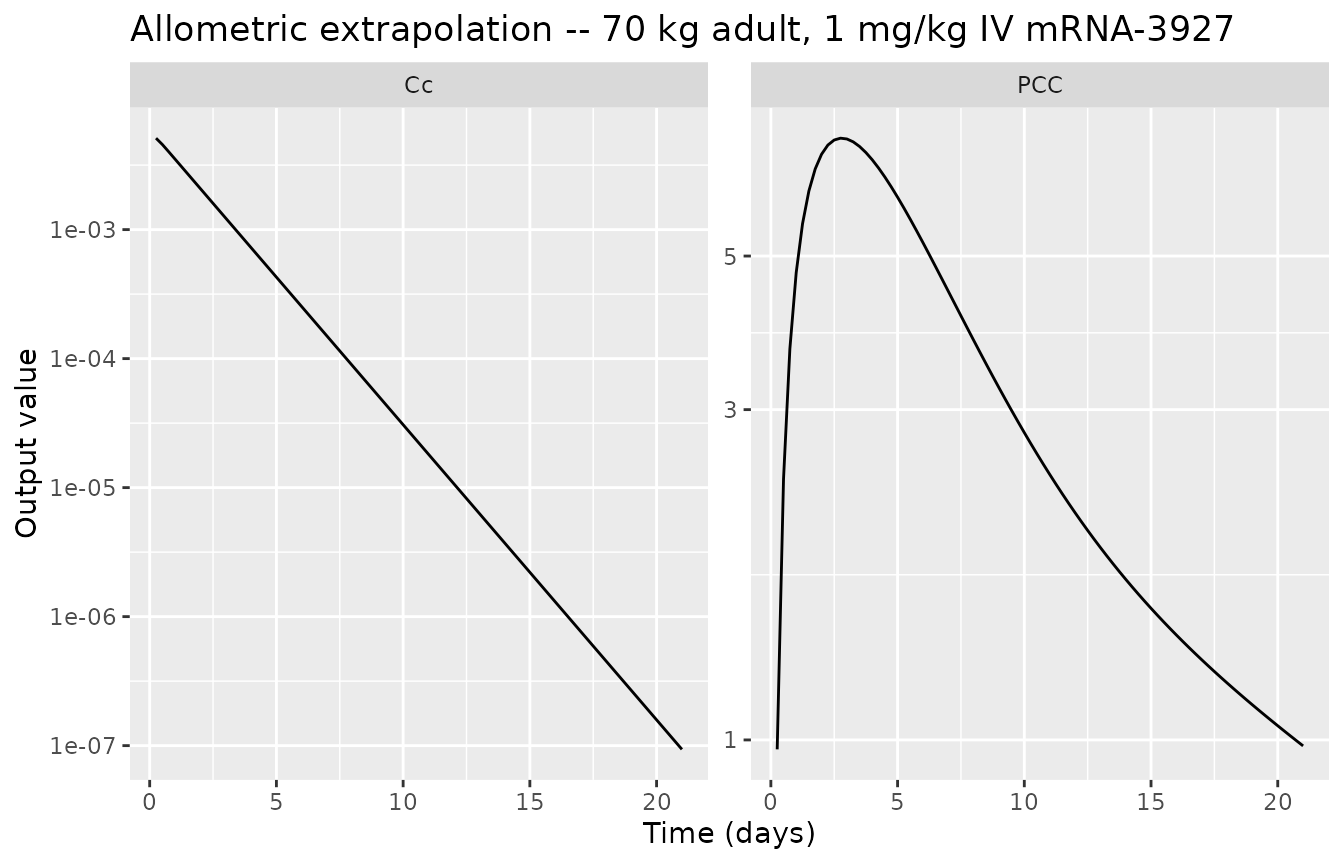

PKNCA validation – plasma PCCA / PCCB mRNA (single-dose, mouse 1 mg/kg)

Attarwala 2023 does not tabulate NCA parameters for plasma mRNA, so this section serves as an internal numerical check that the simulated single-dose PK profile yields plausible NCA metrics rather than a side-by-side comparison against the source.

pknca_t <- c(0.01, 0.25, 0.5, seq(1, 48, by = 1))
pknca_dose <- tibble::tibble(id = 1L, time = 0, amt = 0.025, evid = 1L,
                              cmt = "central", WT = 0.025)
pknca_obs  <- tibble::tibble(id = 1L, time = pknca_t, amt = 0, evid = 0L,
                              cmt = "Cc", WT = 0.025)
pknca_events <- dplyr::bind_rows(pknca_dose, pknca_obs) |>
  dplyr::mutate(treatment = "mouse_1_mgkg") |>
  dplyr::arrange(time, dplyr::desc(evid))

sim_pknca <- rxode2::rxSolve(mod_typical, events = pknca_events,
                              keep = c("treatment")) |>
  as.data.frame() |>
  dplyr::mutate(id = 1L)
#> ℹ omega/sigma items treated as zero: 'etalcl32', 'etale0_mc2', 'etalbase_mc2', 'etale0_hp3', 'etalbase_hp3', 'etale0_c3c2', 'etalbase_c3c2'

conc_df <- sim_pknca |>
  dplyr::filter(!is.na(Cc), time > 0) |>
  dplyr::select(id, time, Cc, treatment)

dose_df <- pknca_events |>
  dplyr::filter(evid == 1L) |>
  dplyr::mutate(treatment = "mouse_1_mgkg") |>
  dplyr::select(id, time, amt, treatment)

conc_obj <- PKNCA::PKNCAconc(conc_df, Cc ~ time | treatment + id)
dose_obj <- PKNCA::PKNCAdose(dose_df, amt ~ time | treatment + id)

intervals <- data.frame(
  start = 0,
  end   = 48,
  cmax  = TRUE,
  tmax  = TRUE,
  auclast = TRUE,
  half.life = TRUE
)

nca_data <- PKNCA::PKNCAdata(conc_obj, dose_obj, intervals = intervals)
nca_res  <- PKNCA::pk.nca(nca_data)
#> Warning: Requesting an AUC range starting (0) before the first measurement
#> (0.01) is not allowed
summary(nca_res)
#>  start end    treatment N auclast    cmax   tmax half.life
#>      0  48 mouse_1_mgkg 1      NC 0.00870 0.0100      6.02
#> 
#> Caption: auclast, cmax: geometric mean and geometric coefficient of variation; tmax: median and range; half.life: arithmetic mean and standard deviation; N: number of subjects

Assumptions and deviations

Supplement equation typo. Supplementary Table S1 (B) writes the central PCC ODE as d(PCC)/dt = Ksyn * Ce + Kq*(PCP - PCC) - Kdeg * PCC with Ksyn = Ce * Slope. Taken literally this is quadratic in Ce, which conflicts with (i) the main text, which states PCC synthesis is “a linear function of plasma PCCA/B mRNA concentration” (p. 143), and (ii) the Slope units (mg/g/h)/(mg/mL), which directly convert Ce (mg/mL) to a synthesis rate (mg/g/h). We implement the linear-in-Ce form: d(PCC)/dt = Slope * Ce + Kq*(PCP - PCC) - Kdeg * PCC.
Compartment names. Per the nlmixr2lib naming convention, plasma 1 (A1) is mapped to central, tissue (A2) to peripheral1, and plasma 2 (A3) to peripheral2. Both plasma compartments share the same volume vc; tissue has its own volume vp. This re-mapping does not change the equations; only the symbol names. The PCC protein central and peripheral PD compartments are named pcc and pcc_p respectively. These two names are not in nlmixr2lib’s canonical compartment list (no entry covers the paper-specific PCC protein pool), so checkModelConventions() emits two compartments warnings, kept here so the names match the paper.
Mouse body-weight reference. The paper writes the allometric scaling as (BW / 0.025)^exp. We supply WT as a user covariate; the scaling reference is the 25 g PCC-deficient mouse the PK was anchored to. Setting WT = 0.025 therefore recovers the typical-value mouse parameters.
IIV interpretation. The published Table 1 reports IIV as a percentage for the seven IIV parameters (CL32 plus two per biomarker). We treat these as CV% and convert via omega^2 = log(1 + CV^2); the converted values are pasted into ini() with the conversion shown in comments.
Fixed parameters. V, V2, and Imax are reported with “Fixed” values in Attarwala 2023 Table 1 (footnotes f and m). All three are wrapped in fixed(...) in ini(). Allometric exponents on volume parameters are also fixed at 1 per Supplementary Table S1.
Species-pooled PK fit, mouse-only PD fit. The published PK model was fit jointly across mouse / rat / monkey using allometric scaling; PD layers (PCC protein and downstream biomarkers) were fit on mouse data only. The packaged model carries the PD layer as published. When simulating non-mouse species the biomarker outputs should be interpreted as the paper’s allometric extrapolation, not direct fits.
No NCA comparison. Attarwala 2023 does not tabulate NCA parameters for plasma mRNA. The PKNCA chunk above is a self-consistency check only.
Variability replication for figure overlays is not attempted. The raw preclinical dataset is not publicly available; we replicate only the typical-individual (population-predicted) curves from Figures 2A and 2B and Supplementary Figures S1-S3, not the per-subject scatter.